Deep Learning vs. Bayesian Knowledge Tracing: Student Models for Interventions

Deep Learning vs. Bayesian Knowledge

Tracing: Student Models for Interventions

Ye Mao

Department of Computer Science North Carolina State University [email protected]

Chen Lin

Department of Computer Science North Carolina State University [email protected]

Min Chi

Department of Computer Science North Carolina State University [email protected]

Bayesian Knowledge Tracing (BKT) is a commonly used approach for student modeling, and Long Short Term Memory (LSTM) is a versatile model that can be applied to a wide range of tasks, such as lan-guage translation. In this work, we directly compared three models: BKT, its variant Intervention-BKT (IBKT), and LSTM, on two types of student modeling tasks: post-test scores prediction and learning gains prediction. Additionally, while previous work on student learning has often used skill/knowledge components identified by domain experts, we incorporated an automatic skill discovery method (SK), which includes a nonparametric prior over the exercise-skill assignments, to all three models. Thus, we explored a total of six models: BKT, BKT+SK, IBKT, IBKT+SK, LSTM, and LSTM+SK. Two training datasets were employed, one was collected from a natural language physics intelligent tutoring system named Cordillera, and the other was from a standard probability intelligent tutoring system named Pyre-nees. Overall, our results showed that BKT and BKT+SK outperformed the others on predicting post-test scores, whereas LSTM and LSTM+SK achieved the highest accuracy, F1-measure, and area under the ROC curve (AUC) on predicting learning gains. Furthermore, we demonstrated that by combining SK with the BKT model, BKT+SK could reliably predict post-test scores using only the earliest 50% of the entire training sequences. For learning gain early prediction, using the earliest 70% of the entire se-quences, LSTM can deliver a comparable prediction as using the entire training sequences. The findings yield a learning environment that can foretell students’ performance and learning gains early, and can render adaptive pedagogical strategy accordingly.

Keywords:student modeling, learning gain, interventions, LSTM, BKT

1. I

The primary objective of this work is to build an analytic model that can both actively track whether a student has embarked upon an unprofitable learning experience and accurately identify those who may fail the corresponding test as early as possible so that adaptive recommendation can be offered. Many existing ITSs areelicit-centric, meaning the system-student interactions can be viewed as a temporal sequence of steps (VanLehn, 2006) in which each step the tutor

elicitsthe subsequent step from the student. This can be done with prompting, but often done without it (e.g., in a free form equation entry window where each equation is a step). When a student enters an attempt on a step, the ITS records whether it is a success or failure and may give feedback and/or hints based on that entry. Students’ first attempts recorded on each step are then extracted for student modeling.

Bayesian Knowledge Tracing (BKT;Corbett and Anderson 1994) is one of the most popular student modeling approaches that keeps track of students’ knowledge over time. Conventional BKT infers students’ hidden knowledge states mainly from their performance (i.e.,correct, in-correct) on each step. Nevertheless, student performance can be noisy because many ITSs allow students to refer to external resources for information. The ability to solicit help from external resources obscures the fact of whether a student has truly learned or not. On the other hand, ever since the mid-1950s, response time has been used as a preferred dependent variable in cognitive psychology (Thomas et al., 1986). Student response time has been mainly used to assess student learning because it can indicate how active and accessible student knowledge is. For example, it has been shown that response time reveals student proficiency (Schnipke and Scrams, 2002) and there is a significant negative correlation between student average response time and student final exam score taken at the end of the semester (Gonz´alez-Espada and Bullock, 2007). Also, response time has been suggested as an indicator of student engagement in answering questions (Beck, 2005) as well as an important factor for predicting motivation in e-learning environments (Cocea and Weibelzahl, 2006). Previously, we explored three types of observations: the con-ventionalperformance, the proposedstudent response time, and thecombinedobservations; our results showed using thecombinedobservation is more effective than using either of them alone (Lin and Chi, 2017). Therefore, in this work, we used both performance and student response time to infer student hidden knowledge level.

Furthermore, much of the prior research on student modeling has been conducted on datasets collected fromelicit-centricITSs. Inelicit-centricITSs (Aleven and Koedinger, 2002;Graesser et al., 2004, for eg. Cognitive Tutor, AutoTutor), the activities are mainly guided by tutors who

elicit the next step from students. However, some ITS are notelicit-centric. For example, the two datasets used in this work were collected from Cordillera and Pyrenees where the tutors are able to choose toelicitthe next step information from students, or totellthem the next step directly (see Figure1). Figure1compares a pair of dialogues extracted from logs in this study. Both dialogues begin and end with the same tutor turn (lines 1 and 6 in (a) and 1 and 4 in (b)). In dialogue (a) the tutor chooses to elicit twice (lines 2-3 and 4-5 respectively). Dialogue (b), by contrast, covers the same domain content with two tell actions (lines 2 and 3). As a consequence, tutorial dialogue (a) is more interactive than (b). In this example, both elicits and tells are

(a) Elicit Version (b) Tell Version

1. T: So let’s start with determining the value of v1.

2. T:Which principle will help you calcu-late the rock’s instantaneous magnitude of velocity at T1?{ELICIT}

3. S:definition of kinetic energy

4. T:Please write the equation for how the definition of kinetic energy applies to this problem at T1{ELICIT}

5. S:ke1 =0.5*m*v1ˆ2

6. T:From KE1 = 0.5*m*v1ˆ2,· · ·

1. T: So let’s start with determining the value of v1.

2. T:To calculate the rock’s instantaneous magnitude of velocity at T1, we will apply the definition of kinetic energy again. {TELL}

3. T:Let me just write the equation for you: KE1 = 0.5*m*v1ˆ2.{TELL}

4. T:From KE1 = 0.5*m*v1ˆ2,· · ·

Figure 1: Elicit vs. Tell

and IBKT. Furthermore, both models were compared against a deep learning based model. Long Short Term Memory (LSTM;Hochreiter and Schmidhuber 1997) is a special type of deep learning model. LSTM is a variant of the Recurrent Neural Network (RNN) that was proposed to solve vanishing and exploding gradient problems (Hochreiter and Schmidhuber, 1997). Therefore, LSTM is effective in capturing underlying temporal structures in time series data, and it captures long-term dependencies more effectively than conventional RNN (LeCun et al., 2015). More specifically, instead of arbitrarily squashing the previous state every step with a sigmoid, LSTM builds up memory by feeding the previous hidden state as an additional input into the subsequent step. This makes the model particularly suitable for modeling dynamic information in student modeling, where there are strong statistical dependencies between student learning events over long-time intervals. In recent years, LSTM has been shown to be able to discover intricate structures in large datasets, achieving state-of-the-art results in a wide range of domains (Graves et al., 2013;Luong and Manning, 2015;Ng et al., 2015;Xingjian et al., 2015). In this work, we implement two Bayesian models, BKT and IBKT, and one deep learning model, LSTM, to model student learning with instructional interventions.

automatically (Lindsey et al., 2014, SK) . In the present study, we explore the impact of using automatically discovered KCs on the effectiveness of the three models. Combining SK with the three models (i.e., BKT, IBKT and LSTM) results in three new variations (i.e., BKT+SK, IBKT+SK, and LSTM+SK). These six models are applied to two important student modeling tasks: 1) predicting students’ post-test scores, and 2) predicting their learning gains.

Post-test scores obtained at the end of training process were used represent students’ learn-ing outcomes: the higher the post-test score, the more likely the student has mastered the knowl-edge. Learning gain, on the other hand, measures how much a student has learned: the higher a student’s learning gain, the more the student benefits from the tutor. Both post-test scores and learning gains are important outcomes for student learning. Note that students with a higher post-test score may not have a higher learning gain and vice versa. Therefore, our goal is to explore which of the six models is more effective at a particular task. Last but not least, we also want to develop a predictive tool that will identify students at high risk of failing the post-test; and those that will fail to benefit from a tutoring system as early as possible. Motivated by this, we investigate two important research questions regarding post-test prediction and learning gain prediction respectively: 1) for the task of post-test score prediction, which of the six models is best: BKT, BKT+SK, IBKT, IBKT+SK, LSTM or LSTM+SK? 2) for the task of learning gain prediction, which of the six models is best? This research sheds some lights on predicting post-test and learning gains and the resulting best models to employ for carrying out adaptive pedagogical strategies, and further advanced personalized learning.

2. R

W

2.1. MODELINGSTUDENT LEARNING

Modeling student cognitive processes is highly complex since it is influenced by many factors such as motivation, aptitude and learning habit. The high volume of features and tools provided by computer-based learning environments confound the task of tracking student knowledge even further. An accurate student model is a building block for any computer-based educational software that provides adaptivity and personalization. Student modeling has been widely and extensively explored in previous research. For example, prior research has proposed a series of approaches based on logistic regression including Item Response Theory (Tatsuoka, 1983), Learning Factor Analysis (Cen et al., 2006), Learning Decomposition (Beck and Mostow, 2008), Instructional Factors Analysis (Chi et al., 2011), Performance Factors Analysis (Pavlik et al., 2009), and Recent-Performance Factors Analysis (Galyardt and Goldin, 2014). These models were implemented with different parameters to better understand and model student learning and were shown to be very successful. In this work, however, we mainly focus on BKT, IBKT and LSTM.

(2013) parameterized student learning rates in BKT models and the results showed that the new model outperformed conventional BKT in predicting whether the students’ next responses were going to be correct/incorrect. Baker et al. (2008) investigated contextualized guess and slip rates to deal with the issues of identifiability and model degeneracy commonly observed in con-ventional BKT. Their results suggested that the proposed models achieved better performance in predicting students’ next-step response than BKT. Pardos and Heffernan (2011) introduced problem difficulty to BKT and found substantial performance improvement in predicting stu-dent step-by-step responses over BKT. In short, BKT and BKT-based models have been shown to be effective in many student modeling tasks. While previous studies mainly applied BKT to

elicit-centricITSs, our studies applied BKT based models to ITSs involving multiple instruc-tional interventions. Addiinstruc-tionally, previous studies used students’ performance (i.e., correct, incorrect) as observations, whereas we used both performance and student response time as observations for training the BKT based models.

In our prior work,Lin and Chi (2016) proposed Intervention-BKT (IBKT) that incorporates tutor’s intervention (e.g., elicit and tell). Our proposed model outperformed conventional BKT in post-test score prediction, and demonstrated great potential in providing personalized inter-vention. Lin et al. (2016) further incorporated the effect of student response time to IBKT. The proposed IBKT model was applied to predict students’ next-step responses and post-test scores and demonstrated great improvement over conventional BKT.

The Bayesian family models are straightforward and robust. Nonetheless, it’s inherently difficult to fully capture the complexity and diversity of data due to its restricted functional form as a graphical model. On the other hand, deep neural network based approach such as recurrent neural network (RNN) exhibits greater flexibility compared to BKT-based models. First, they do not require explicitly encoded domain concepts. Second, they allow multivariate inputs as long as each variate can be vectorized. Finally, they are capable of learning long-term dependencies modeling complicated rules without many assumptions or prior knowledge from human experts. LSTM is a variation of RNN that addresses the exploding and vanishing gradient problems commonly observed in RNN. These deep recurrent models have shown great success in many domains such as speech recognition (Graves et al., 2013), language translation (Luong and Manning, 2015), video classification (Ng et al., 2015), and rainfall intensity prediction (Xingjian et al., 2015), etc. Their success in all these domains has opened up a new line of research in educational data mining (Piech et al., 2015; Tang et al., 2016;Khajah et al., 2016;

Wilson et al., 2016; Xiong et al., 2016; Lin and Chi, 2017). For example, Lin and Chi (2017) compared both RNN and LSTM against conventional BKT to predict student learning gains and found deep learning-based models have superior performance. For the task of predicting students’ responses to exercises, LSTM was shown to outperform conventional BKT (Piech et al., 2015) and Performance Factors Analysis (Pavlik et al., 2009). However, RNN and LSTM did not always have better performance when the simple, conventional models incorporated other parameters (Khajah et al., 2016;Wilson et al., 2016).

2.2. KNOWLEDGE COMPONENT DISCOVER OR SKILL DISCOVERY (SK)

In the intelligent tutoring literature, it is commonly considered that relevant knowledge in do-mains such as math and science is structured as a set of independent but co-occurring Knowledge Components (KCs). It is assumed that the student’s knowledge state at one KC has no impact on the student’s understanding of any other KCs. This is an idealization, but it has served ITS de-velopers well for many decades and is a fundamental assumption made by many student models (Corbett and Anderson, 1994). Therefore, determining the set of skills or knowledge compo-nents required to solve a step, a problem, or an exercise is of great importance regardless of what models are used.

Cen et al. (2006) proposed Learning Factors Analysis (LFA) to improve the cognitive model by splitting or merging the KCs based on expert-identified difficulty factors. Although this method achieved better statistical scores and is highly interpretable, it heavily relies on domain expertise. Gonz´alez-Brenes and Mostow (2012) proposed a fully automatic method – Dynamic Cognitive Tracing, which achieved a comparable estimate on true cognitive model from which the synthetic data was created; however, it does not scale well due to the fact that both the memory and run-time grow exponentially with the number of items and skills, respectively.

Barnes (2005) applied Q-matrix method to explore the question-concept relationships based on student responses; however, one assumption of the Q-matrix is that student knowledge states are static. This assumption does not often hold as students can learn from question to question when training on ITSs.

3. M

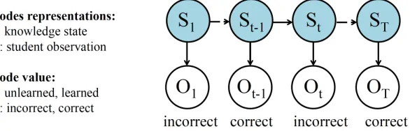
BKT is a student modeling method extensively used in ITS. Figure2 shows a graphical repre-sentation of the model and a possible sequence of student observations. The shaded nodes S

represent hidden knowledge states. The unshaded nodesO represent observation of students’

behaviors. The edges between the nodes represent their conditional dependence.

Figure 2: The Bayesian network topology of the standard Knowledge Tracing model

Fundamentally, the BKT model is a two-state Hidden Markov Model (HMM; Eddy 1996) characterized by five basic elements: 1)N, the number of different types of hidden state; 2)M, the number of different types of observation; 3)Π, the initial state distributionP(S0); 4)T, the

state transition probability P(St+1|St)and 5) E, the emission probability P(Ot|St). Note that

both N and M are predefined before training occurs, while Π, T and E are learned from the

students’ observation sequence.

Conventional BKT assumes there are two types of hidden knowledge state (N=2) corre-sponding to student knowledge states ofunlearned andlearned. It also assumes there are two types of student observation (M=2) correspondint to student performance ofincorrectand cor-rect. BKT makes two assumptions about its conditional dependence as reflected in the edges in Figure2. The first assumption BKT makes is a student’s knowledge state at a timetis only

contingent on her knowledge state at timet₋1. The second assumption is a student’s

perfor-mance at timet is only dependent on her current knowledge state. These two assumptions are

captured by the state transition probabilityTand the emission probabilityE. To fit in the context of student learning, BKT further defines five parameters:

Prior Knowledge= P(S0=learned)

Learning Rate= P(learned_|unlearned ) Forget= P(unlearned_|learned)

Guess= P(correct|unlearned)

Slip= P(incorrect_|learned)

Baum-Welch algorithm (or EM method) is used to iteratively update the model’s parameters until a maximized probability of observing the training sequence is achieved.

3.2. INTERVENTION-BKT

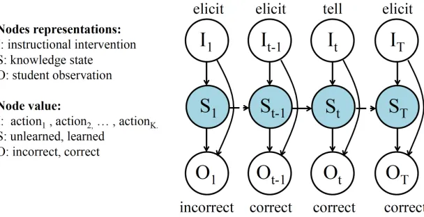
observation nodes O represent how instructional interventions affect a student’s performance.

The arrows between input nodes I and knowledge state nodes S represent how instructional

interventions affect a student’s hidden knowledge state.

Figure 3: The Bayesian network topology of the Intervention-BKT model

Intervention-BKT is a special case of Input Output Hidden Markov Model (Marcel et al., 2000), which is extended from HMM. This model is characterized by six basic elements: 1)K, the number of different types of input; 2)N, the number of different types of hidden state; 3)M, the number of different types of observation; 4)Π, the initial state distributionP(S0); 5)T, the

state transition probabilityP(St|It, St₋1), and 6)E, the emission probabilityP(Ot|It, St)

Intervention-BKT makes two distinctions compared to BKT. First, it employs a parameter K representing the number of input types, that is, the instructional intervention types. Second, Intervention-BKT makes two different assumptions about its conditional dependence as repre-sented by the edges in Figure3: 1) a student’s knowledge state at a timetis contingent on her

previous state at timet₋1as well as the current interventionIt, and 2) a student’s performance at timetis dependent on her current knowledge stateStas well as the current interventionIt. Similarly, Our Intervention-BKT employs1+4_×Kparameters (compared with 5 parameters of

BKT) to describe its conditional probability. ThePrior Knowledgeshare the same definition as conventional BKT:Prior Knowledge= P(S0=learned). For each of the K types of interventions

Aj, j ∈[1, K], Intervention-BKT defines four parameters:

Learning RateAj = P(learned|unlearned,It=Aj ) Forget_Aj = P(unlearned_|learned,It =Aj)

GuessAj= P(correct|unlearned,It=Aj) Slip_Aj = P(incorrect_|learned,It =Aj)

In this work, we mainly focus on modeling two types of instructional interventionelicitand

3.3. LSTM

LSTM (Hochreiter and Schmidhuber, 1997) is a special type of RNN which is explicitly de-signed to avoid the long-term dependency problem, and was refined and popularized by many people in recent works (Gers et al., 1999; Gers and Schmidhuber, 2000; Gers and Schmidhu-ber, 2000; Kalchbrenner et al., 2015; Xu et al., 2015). LSTM can avoid the vanishing (and exploding) gradient problem and work tremendously well on a large variety of problems.

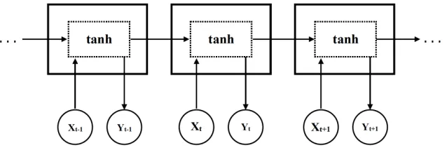
Figure 4: The network structure of an RNN (Xtrepresents input;Ytrepresents output)

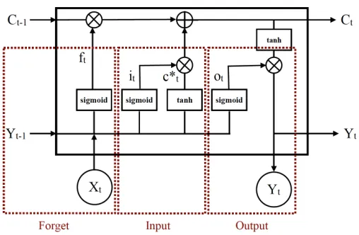
All recurrent neural networks have the form of a chain of repeating modules of neural net-work. In standard RNNs, this repeating module will have a very simple structure, such as a single tanh layer, as shown in Figure4. LSTMs also take the form of a chain like structure, but the repeating module has a different structure. The internal structure of each LSTM module is shown in Figure5. Instead of having a single neural network layer, there are three major compo-nents including Forget, Input, and Output, thus resulting in a more complex structure than RNN. These components interact with each other to control how information flows.

In the first step, a function of the previous hidden state and the new input passes through the forget gate, indicating what is probably irrelevant and can be taken out of the cell state. The forget component will calculate a weight ft between 0 to 1 for each element in hidden state

vectorCt−1. An element with a weight of 0 should be completely forgotten whereas an element

with a weight of 1 needs to be entirely remembered. The formula to calculateftis shown below

whereWf andbf are the weights and intercept, respectively for the forget component.

ft=sigmoid(Wf _·[Yt₋1, Xt] +bf) (1)

There are two steps involved in Input component’s calculation. In the first step, a tanh layer calculates a candidate vector C∗

t that could be added to the current hidden state. In the second

step, the input components calculate a weight vector it (ranging from 0 to 1) to determine to

what extendCt∗ should update the current memory state.

C_t∗ = tanh(WC ·[ht₋1, xt] +bc) (2)

it=sigmoid(Wi_·[Yt₋1, Xt] +bi) (3)

Figure 5: The network architecture within a LSTM module

computingC∗

t ·it. Consequently, the formula to update the current memory cell is shown below.

Note that the current memory cell stateCtis then passed to the next LSTM module.

Ct=Ct₋1·ft+Ct∗·it (4)

Finally, the output component is simply an activation function that filters elements in Ct.

TheCtcan be converted to a value between -1 to 1 by thetanhfunction. The output component

calculates a weight vector

Ot=sigmoid(Wa·[Ht−1, Xt] +bo) (5)

that determines how much information is allowed to be revealed.

Yt=Ot∗tanh(Ct) (6)

To apply LSTM to our task, each student’s trajectory can be seen as{< X1, ...Xi, ..., XT >

, Y}whereT is the total number of steps,Xiis the input for a given student at timestampi, and Y is the output: the student’s post-test score or learning gain. More specifically,Xicontains the

following features: 1) the skills (either designed by the expert or discovered by the SK) involved in the stepi, 2) the corresponding instructional intervention determined by the tutor (e.g.,elicit

ortell), 3) the student’s performance on the step (e.g.,correctorincorrect), and 4) the student’s response speed (e.g.,fastorslow).

3.4. AUTOMATIC SKILL DISCOVERY

WCRP is an extension of Chinese restaurant process (CRP;Aldous 1985), which describes a scenario in which each entering customer needs to choose a table, and each customer has a fixed affiliation and prefers to sit at tables with customers having similar affiliations. In the mapping of the WCRP to our domain, customers correspond to exercises, tables to distinct skills, and affiliations to expert labels. Thus, in our prediction tasks, we need to assign a skill to each exercise, which carries its affiliation towards the expert-identified skills. Xi denotes the expert

label associated with exercisei, andYirepresents the skill assigned to exercisei. The probability

an occupied skilly∈ {1, ..., Nskill}is chosen when a new exercise is observed is specified via:

P(Yi =y|Xi,X(y))∝ny 1 +β(κ xi

y −1)

1 +β(Nskill−1₋1) (7)

where X(y) _{is the set of affiliations of exercises assigned to skill y and n}

y is the number of

exercises assigned to skilly. β is the previously mentioned bias, an exercise is equally likely

to have any affiliation when β = 0 and all exercises of a skill will take the skill’s affiliation if

β = 1. κα

y is a softmax function that tends toward 1 ifαis the most common affiliation among

exercises of skilly, and tends toward 0 otherwise. In the WCRP, a new skillNskill+ 1is selected

with probability:

P(Yi =Nskill+ 1) ∝α (8)

Hereαis defined asα =α0(1−β)and thusα0 is free to modulate the expected number of the

occupied skills while the term1₋β is constricted to assign new skill when the bias is high.

The conditional probability for Yi given the other variables is proportional to the product

of the WCRP prior term and the joint likelihood of each students response sequence, where Equations 7 and 8 provide the former. For an existing table, the likelihood is given by the BKT HMM emission sequence probability. For a new table, an extra step is required to calculate the emission sequence probability because the BKT parameters do not have conjugate priors. The formula 8 from (Neal, 2000) is adopted here, and it efficiently produces a Monte Carlo approximation of the intractable data likelihood, linking BKT parameters for the new table.

Formally, the method assigns each exercise label to a latent skill such that a students ex-pected accuracy on a sequence of same-skill exercises improves monotonically with practice (Lindsey et al., 2014). In place of discarding the expert-provided skills, the method incorporates a nonparametric prior to the exercise-skill assignments that are based on the expert-provided skills and WCRP.

4. E

4.1. TRAINING DATASETS

4.1.1. Cordillera

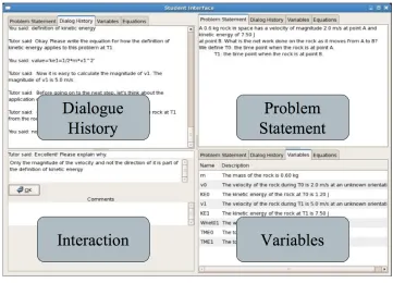
Cordillera (Figure 6) is a natural language ITS for college-level introductory physics. Five domain experts identified 7 primary KCs, and they labeled each step with corresponding KCs, kappa>0.8. All participants in our training corpus went through the following procedures: 1)

completed a survey, 2) read a textbook, 3) took a pretest, 4) solved seven training problems, and 5) took a post-test at the end.

Figure 6: The Cordillera Interface

In total, there are 44,323 data points from 169 students. Each student completed around 300 training problem steps. A data point in our training dataset is either the first student attempt in response to a tutor elicit, or a tutortell indicating the next step. The pretest and post-test have the same 33 test items. All of the tests were graded in a double-blind manner by a single domain expert (not the authors). Each test question was assigned two types of grades: an overall grade and a KC-based grade. The overall grade was a score in the range [0, 1] describing the correctness of an answer as a whole, while the KC-based grade was a score in the same range describing the correctness regarding a particular KC.

4.1.2. Pyrenees

Overall, Pyrenees’ dataset is comprised of 68,740 data points from 475 students. Pyrenees is a web-based ITS teaching probability, which covers 10 major KCs, such as the Addition Theorem, the Complement Theorem, and Bayes Rule, etc. Domain experts both identified the 10 KCs and labeled each step/exercise with the corresponding KCs, kappa > 0.9. Figure 7shows the

the next step. Students can enter their inputs in the text area. Any variable or equation that is defined through this process is displayed on left side of the screen for reference. In Pyrenees, whenever an answer is submitted, the tutor provides immediate feedback. In addition to this, Pyrenees can also provide on-demand hints. The bottom-out hint tells the student exactly how to solve a problem.

Figure 7: The Pyrenees Interface

When training on Pyrenees, students were required to complete 4 phases: 1) pre-training, 2) pretest, 3) training, and 4) post-test. During the pre-training phase, all students studied the do-main principles from a probability textbook. The students then took a pretest which contained 10 problems. The textbook was not available. They were not given feedback on their answers, nor were they allowed to go back to earlier questions. During the training phase, students received the same 12 training problems in the same order on Pyrenees. Each domain concept was applied at least twice. The minimum number of steps needed to solve each training problem ranged from 10 to 50. The number of domain principles required to solve each problem ranged from 3 to 11. Finally, all of the students took a post-test with 16 problems. As with Cordillera, both pretests and post-tests were graded in a double-blind manner by a single experienced grader. The scores were normalized using a range of [0,1].

4.2. QUANTIZED LEARNINGGAIN

In our study, the models were not only applied for post-test scores prediction, but also learning gains prediction. We argue the latter is much more challenging because students who perform well in the pretest or during the training often perform well in the post-test, but may or may not benefit from the tutor. For example, on both datasets used here, we found a significant strong positive correlation between students’ pre- and post-test scores: r =0.76andp=4.60_×10−33

for Cordillera, andr=0.673andp=6.04×10−46_{for Pyrenees respectively; however, no strong}

correlation was found between students’ pretest and Normalized Learning Gain: r=−0.04and

p=0.607for Cordillera, andr=₋0.02andp=0.683for Pyrenees.

The concept oflearning gainis formally defined as the difference between the skills, com-petencies, content knowledge and personal development demonstrated by students at two points in time (McGrath et al., 2015). Many studies usedLearning Gain (LG), calculated asLG =

Figure 8: Quantized Learning Gain

2007). A widely used adjusted measurement,Normalized Learning Gain(NLG) was proposed to ensure a consistent analysis over a population with different levels of proficiency: NLG =

post−pre

1−pre (Hake, 2002) where 1 is the maximum score for pre- and post-tests. Fundamentally, the

NLG can be seen as how much a student improves from pretest to post-test (post₋pre) divided

by how much he/she can improve (1−pre). The values of NLG range from (-∞, 1]. A negative NLG occurs when a student gets higher pretest score than post-test score. Thus, NLG can be problematic for students with high pretest scores in that even a modest decline in post-test score from the pre-test can result in large negative NLG. For example, a student who scored 0.99 in the pretest and 0.95 in the post-test would have an NLG of−4 while if he/she scored 0.95 in

the pretest and 0.99 in the post-test would have an NLG of0.8. Such asymmetry is one of the

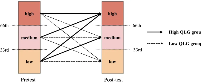
main criticisms of using NLG. Therefore, we used a qualitative measurement calledQuantized Learning Gain(QLG;Lin and Chi 2017) to determine whether a student has benefited from a learning environment.

Our QLG is a binaryqualitative measurement on students’ learning gains from pretest to the posttest: High vs. Low. To infer QLGs, students were split into low, medium, and high based on whether they scored below the 33rd percentile, between the 33rd and 66th percentile, or higher than the 66th percentile in pre-test and post-test respectively. Once a student’s pre- and post-test performance groups are decided, the student is a “High” QLG if he/she moved from a lower performance group to a higher performance group from pre-test to post-test or remained in “high” performance groups; whereas a “Low” QLG is assigned to the student if he/she either moved from a higher performance group to a lower performance group from pre-test to post-test, or stayed at a “low” or “medium”groups (as shown in Figure8). In Figure 8, solid lines represented the formation of theHighQLG groups and dashed lines represents the formation of theLowQLG groups, and they will be coded with “1” and “0” respectively for QLG prediction.

4.3. MODELS CONFIGURATION

from original study (Lindsey et al., 2014) were adopted and fed to the two datasets used. We focused on two prediction tasks. The first task was to predict their post-test scores, referred to as “post-test scores predictions”. The second task was to predict their Quantized Learning Gain (QLG), referred to as “learning gain predictions”.

Unlike the conventional BKT family models, which only use students’ performance (e.g.,

correct and incorrect), we also included their speed of response. It is denoted by one of two symbols: quick and slow. The symbols were assigned by comparing the student’s response time on that step with the median response time of all students on the same step. If the time is greater than the median, we classify it asslow, otherwise,quick. Thus, we combined students’ performance and speed, resulting in four different values:correct-quick,correct-slow, incorrect-quick, andincorrect-slow. Following the classic BKT assumption that students never forget the knowledge once they have learned it, we also setP(unlearned|learned) = 0 for all the BKT

based models in this study.

To train BKT based models, two steps were involved. In the first step, the probability of a student being in thelearnedstate on each KC at the last attempt was learned from the BKT/IBKT models. In the second step, the output of the first step was computed as features for our pre-diction tasks. That is, the number of features involved here equals to the total number of KCs involved. Linear regression and logistic regression were applied to predict post-test scores and QLG respectively. Here linear regression and logistic regression are selected as our prediction models because they are the activation functions used by LSTM models to predict the post-test scores and QLG respectively (described in next paragraph). Additionally, we also compared linear regression and logistic regression against other popular models such as Support Vector Machine, and the former two had better performance, therefore, they are used for comparing BKT based models with LSTM based ones.

To train LSTM, sequences of tuples representing student-system interactions were extracted. The tuples consist of four elements: 1) the assignment of KCs, 2) the instructional interventions, 3) the student response time, and 4) performance. Instead of directly applying an existing LSTM module, we explored the effectiveness of two-layer LSTM with an output layer to make a final prediction. The same as the BKT based models, linear was selected for post-test prediction and sigmoid was used for QLG prediction. Different numbers of units ranging from 5 to 200 were tested and the best model was chosen based on the 5-fold cross-validation results. We also applied early stopping callbacks to avoid the potential overfitting problem.

5. R

5.1. AUTOMATIC SKILL DISCOVERY RESULTS

The overall results from automatic skill discovery are presented in Table1. The columnDataset

Table 1: Results of the SK Discovery Method

Dataset Students Items Expert Skills Discovered Skills

Cordillera 169 1187 7 24

Pyrenees 475 176 10 15

Furthermore, some preliminary explorations on the skills discovered by the SK method showed that they are indeed different from the expert labels. For example, in Pyrenees, the expert originally labeled both P(D|B) andP(D|A∩B ∩C)with the same KC, “the Bayes

rule”. However, two different KCs were assigned to them by SK, more specifically, “the Bayes rule to an atomic event” is assigned toP(D_|B)while “the Bayes rule to a combination of events”

is assigned toP(D|A∩B∩C).

5.2. POST-TEST PREDICTION

5-fold cross-validation Root Mean Square Error (RMSE) was used to evaluate the models (Table

2). RMSE measures the difference between the predicted post-test scores and the actual post-test scores: the lower the value, the higher the predictive accuracy.

5.2.1. Comparison between Models

Table 2: RMSE in Post-test Score Prediction

Model _{Cordillera Pyrenees}Data

Non-SK models

1 BKT 0.147* 0.162

2 IBKT 0.177 0.168

3 LSTM 0.183 0.179

SK models

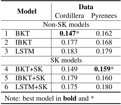
4 BKT+SK 0.149 0.159* 5 IBKT+SK 0.179 0.160 6 LSTM+SK 0.175 0.180 Note: best model inboldand *

Table2shows the performance of the six models on the post-test score prediction using the entire student training trajectories on the corresponding ITS. The best model is labeled inbold

On the other hand, it was not very clear how much SK helps for each model when using the entire sequences to predict students’ post-test scores. Overall, the improvement of using SK over using the expert-designed KCs can be negligible. For the three basic models, sometimes SK can help: LSTM+SK outperformed LSTM for Cordillera, BKT+SK and IBKT+SK outperformed BKT and IBKT respectively for Pyrenees. But sometimes SK can even reduce the performance: BKT+SK is worse than BKT, IBKT+SK is worse than IBKT for Cordillera and LSTM+SK is worse than LSTM for Pyrenees.

5.2.2. Early Prediction on Post-test Scores

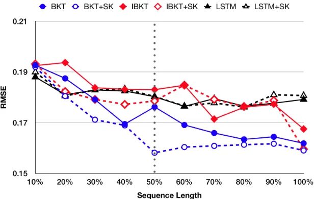
Figure 9: RMSE for Post-test Early Prediction On Cordillera

Figure 10: RMSE for Post-test Early Prediction On Pyrenees

Next, we investigated all the models’ power on post-test score early prediction. Figure 9

BKT models are in blue with circular symbols, IBKT models are in red with square symbols, and LSTM models are in black with triangular symbols. Solid lines with solid symbols represent basic models (BKT, IBKT, and LSTM), and dashed lines with blank symbols represent models with SK (BKT+SK, IBKT+SK and LSTM+SK). The y-axis is the RMSE and the x-axis is the sequence length used for early prediction.

While BKT and BKT+SK perform similarly when using the entire sequences, Figure9and Figure10show that BKT+SK is the best model. Indeed, it outperforms the other models sub-stantially which is evident by the fact that BKT+SK outperformed all the other models starting from 20% all the way to 100%. The results are consistent with both tutoring systems.

More importantly, for both tutoring systems, BKT+SK can predict post-test scores using only 50% of the sequences as effectively as using the entire sequences. Take Cordillera as an example (Figure 9), the RMSE is improved from 10% to 40% (0.186 to 0.155); from 40% to 50%, the improvement becomes moderate (0.155 to 0.149); from 50% to the remaining of the sequences, there is no improvement (0.149 to 0.149). A similar pattern is observed for Pyrenees (Figure10). From 10% to 50%, the RMSE decreases gradually as more observations become available (from 0.192 to 0.158); however, from 50% to 100%, the RMSE is seemingly stabilized (from 0.158 to 0.159). For BKT, on the other hand, it does not predict post-test scores as reliably as using the entire sequences when using the Cordillera dataset. The same is true when 80% of the entire sequences are used for Pyrenees.

In short, our early prediction results clearly show the benefits of using SK. Most notably, BKT+SK achieves the best results: it reliably predicts post-test scores using only 50% of the training sequences for both systems.

5.3. QLG PREDICTION

For QLG prediction, we are primarily interested in identifying students withlowlearning gain. This is because we believe it is more important to recognize those who do not benefit from the tutor preferably as soon as possible since these students may have benefited from the system if other interventions were available.

5-fold cross-validation accuracy, recall, F1-measure, and AUC are reported in Table 3 for QLG prediction. Accuracy measures the fraction of correctly classified students; recall measures the fraction of low learning gain students that are correctly retrieved by the models; F1-measure is the weighted average of recall and precision (measuring the percentage of the predicted low learning gain students whose learning gain is indeed low) and thus F1-measure tells us how robust the model is; and AUC measures the ability of models to discriminate low learning gain students from the high group. For all measurements, the closer to 1, the better.

5.3.1. Comparison between Models

Table 3: QLG Prediction Results on Cordillera and Pyrenees for All Seven Models

Model Accuracy Recall F1-measure AUC

1 Majority 0.544 - - 0.5

Non-SK models

2 BKT 0.663 0.641 0.674 0.665

3 IBKT 0.615 0.761* 0.683 0.601 4 LSTM 0.740* 0.739 0.756* 0.740

SK models

5 BKT+SK 0.674 0.739 0.712 0.668 6 IBKT+SK 0.633 0.685 0.670 0.628 7 LSTM+SK 0.740* 0.696 0.744 0.744* Note: best model inboldand *

(a) Cordillera dataset

Model Accuracy Recall F1-measure AUC

1 Majority 0.562 - - 0.5

Non-SK models

2 BKT 0.665 0.685 0.697 0.662

3 IBKT 0.659 0.749 0.712 0.646

4 LSTM 0.724 0.790* 0.763 0.715 SK models

5 BKT+SK 0.682 0.674 0.705 0.683 6 IBKT+SK 0.665 0.783 0.724 0.649 7 LSTM+SK 0.733* 0.772 0.765* 0.727* Note: best model inboldand *

(b) Pyrenees dataset

Pyrenees. Therefore, among the three basic models BKT, IBKT, and LSTM, LSTM has the best performance for both tutoring systems.

Comparing models using SK, again, LSTM+SK generally has the best performance for both tutoring systems. When comparing LSTM and LSTM+SK, it seems that SK improves accuracy and AUC, but not on recall. On both datasets, LSTM+SK performs worse than LSTM on recall, which may also explain the decline of the F1-measure in Cordillera.

5.3.2. Early Prediction of QLG

the better.

Figure11shows the six model’s performances on the early prediction of QLG for Cordillera. Figure11shows that two LSTM models in black (LSTM, LSTM+SK) outperform the other four Bayesian models at most points across the x-axis on Cordillera. Between the two LSTM models, LSTM (solid black) seems to be more powerful than LSTM+SK (dashed black) espe-cially between 20% to 40%, while LSTM+SK has better F1-measure between 50% to 70%. For the LSTM model, both AUC and F1-measure increase from 10% to 40%: from 0.576 to 0.689 for AUC and from 0.688 to 0.720 for F1-measure; the increase becomes moderate (from 0.688 to 0.746 for AUC; from 0.720 to 0.738 for F1-measure) from 40% to 70%, and finally there is only a slight increase on F1-measure (from 0.738 to 0.756), and a slight decrease on AUC (from

(a) AUC

(b) F1-measure

(a) AUC

(b) F1-measure

Figure 12: AUC and F1-measure for Low QLG Detection On Pyrenees

0.746 to 0.740) between 70% to 100%. The results suggest that areasonableprediction of QLG can be accomplished by using the first 40% of the entire sequences, and that using the earliest 70% of the sequences is as good as using the entire sequences.

30% of the sequence. Note that this results only hold for Pyrenees dataset.

Additionally, from 70% to 100%, the two LSTM models outperform other models, and when using 70% of the entire sequences, the LSTM reach a similar result (0.714 on AUC and 0.755 on F1-measure) compared to the results of using the entire sequences.

6. D

, L

,

F

W

In this work, we investigated three basic student models: BKT, IBKT, and LSTM, as well as their SK variants: BKT+SK, IBKT+SK, and LSTM+SK. Among the six models, four of them belong to the Bayesian family (BKT, BKT+SK, IBKT, and IBKT+SK), and the other two fall in the deep learning group (LSTM, LSTM+SK). The effectiveness of these models was tested using two training datasets involving instructional interventions. The models were applied to two different student modeling tasks: post-test scores and learning gains.

For the task of post-test score prediction, while BKT and BKT+SK are the best models when using the entire training sequence, BKT+SK is shown to be the best model for post-test early prediction. BKT+SK can reliably predict post-test scores when the earliest 50% of its training sequence is used and the result is comparable to using the entire sequence for both training datasets. One potential explanation is that the SK method tends to enrich the skill set and generate more skills than expert KC models which may also be a better model for the domain. Since the performance of BKT models generally heavily depends on the effectiveness of KC models, it can explain why BKT+SK outperformed BKT models on the early prediction of post-test scores.

For the task of the QLG prediction, LSTM and LSTM+SK are the best two models when the entire sequence is used and LSTM is the best model for QLG early prediction as it can reliably predict QLG. Using the earliest 70% of the training sequences, LSTM achieves similar performance as when the entire sequence is used. Back to the internal structure of these models, LSTM is much more complicated than BKT and IBKT, which enables it to capture the changes of students’ learning state better. And we believe that LSTM is able to discover the hidden information that BKT-based models missed and also it explains why the SK method did not help much here.

Overall, we make the following contributions: 1) our work compared the effectiveness of Bayesian based models and deep neural network-based models on two important student mod-eling tasks: post-test scores and learning gains prediction, 2) we explored the robustness and the effectiveness of the proposed models onearly predictiontasks for both post-test scores and learning gains on two training datasets involving different instructional interventions, and 3) for both Bayesian based models and deep neural network based models, we explored the impact of using automatically discovered KCs.

Additionally, here we explored two important student modeling tasks: post-test scores and QLG predictions, but these two scores are not always available for many public educational datasets. So, a general method is needed for handling datasets without these scores. Moreover, both of the two datasets in this work involve two instructional interventions: elicit andtell. It is not clear whether the same conclusions still hold for datasets involving either only one of the interventions (e.g., elicit only) or other types of interventions, such asskip(elicita question without asking students for responses) andjustify(ask students to explain after they provide an answer).

Moreover, we can further improve our models by defining better observation symbols. In our work, we split students’ response time into two levels: fastandslowand a more reasonable approach may be splitting it into three levels: fast, normal, andslow. Also, we applied QLG to instantiate students’ learning gains, which also has some limitations. For example, the current QLG definition would label a student who scored 1% and 32% in the pre- and post-test as Low QLG, the same category as another student who scored 32% and 30% in the pre-test and post-test respectively even though the performance of the former student improved while the performance for the latter student decreased. In future work, we can come up with a composite score including QLG and other metrics, e.g., NLG, to measure students’ learning gain with greater accuracy.

Finally, we will continue to investigate the automatic skills discovered in this work and to improve our SK method. The current SK method heavily relied on the labels from domain ex-perts, so it is not clear whether it can fully recover or even outperform the expert labels if starting from scratch. On the other hand, the interpretability of the latent discovered skills has not been fully explored and further work is needed. Finally, compared with the high interpretability of BKT based models, it is more challenging to interpret the learned LSTM models and what fac-tors are indeed impact student learning gains. Moreover, in this work, the hyperparameters such as the number of neurons in each layer was manually tuned. For future work, we will not only explore how to tune hyperparameters through a more systematic approach, but also investigate the following questions: 1) how to determine what patterns are predictable for students’ learn-ing gain through the trained parameters; 2) how to predict students’ learnlearn-ing gain at a very early stage when few observations are available and suggest effective intervention accordingly.

7. A

This material is based upon work supported by the National Science Foundation under Grant No. 1432156 “Educational Data Mining for Individualized Instruction in STEM Learning En-vironments, 1660878 “MetaDash: A Teacher Dashboard Informed by Real-Time Multichannel Self-Regulated Learning Data”, 1651909 “CAREER: Improving Adaptive Decision Making in Interactive Learning Environments, and 1726550 “Integrated Data-driven Technologies for In-dividualized Instruction in STEM Learning Environments”.

8. E

S

R

ALDOUS, D. J. 1985. Exchangeability and related topics. In ´Ecole d’ ´Et´e de Probabilit´es de Saint-Flour

XIII — 1983, P. L. Hennequin, Ed. Springer, 1–198.

ALEVEN, V. A.ANDKOEDINGER, K. R. 2002. An effective metacognitive strategy: Learning by doing

and explaining with a computer-based cognitive tutor.Cognitive science 26,2, 147–179.

BAKER, R. S., CORBETT, A. T.,ANDALEVEN, V. 2008. More accurate student modeling through

con-textual estimation of slip and guess probabilities in Bayesian knowledge tracing. InProceedings of the

9th international conference on Intelligent Tutoring Systems, B. P. Woolf, E. A¨ımeur, R. Nkambou,

and S. Lajoie, Eds. Springer, 406–415.

BARNES, T. 2005. The q-matrix method: Mining student response data for knowledge. InAmerican

Association for Artificial Intelligence 2005 Educational Data Mining Workshop. 1–8.

BECK, J. E. 2005. Engagement tracing: Using response times to model student disengagement. In Ar-tificial Intelligence in Education: Supporting Learning Through Intelligent and Socially Informed

Technology, C.-K. Looi, G. McCalla, and B. Bredeweg, Eds. IOS Press, 88–95.

BECK, J. E.ANDMOSTOW, J. 2008. How who should practice: Using learning decomposition to

eval-uate the efficacy of different types of practice for different types of students. InIntelligent Tutoring

Systems, B. P. Woolf, E. A¨ımeur, R. Nkambou, and S. Lajoie, Eds. Springer, 353–362.

CEN, H., KOEDINGER, K., AND JUNKER, B. 2006. Learning factors analysis – a general method for

cognitive model evaluation and improvement. InIntelligent Tutoring Systems, M. Ikeda, K. D. Ashley, and T.-W. Chan, Eds. Springer, 164–175.

CHI, M., KOEDINGER, K. R., GORDON, G. J., JORDON, P., AND VANLAHN, K. 2011. Instructional

factors analysis: A cognitive model for multiple instructional interventions. InProceedings of the 4th

International Conference on Educational Data Mining, M. Pechenizkiy, T. Calders, C. Conati, C. R.

Sebastian Ventura, and J. Stamper, Eds. 61–70.

COCEA, M.AND WEIBELZAHL, S. 2006. Can log files analysis estimate learners’ level of motivation?

In LWA 2006: Lernen - Wissensentdeckung - Adaptivitat, 14th Workshop on Adaptivity and User

Modeling in Interactive Systems (ABIS 2006). Number 1/2006 in Hildesheimer Informatik-Berichte.

University of Hildesheim, Institute of Computer Science, 32–35.

CORBETT, A. T.ANDANDERSON, J. R. 1994. Knowledge tracing: Modeling the acquisition of

proce-dural knowledge.User modeling and user-adapted interaction 4,4, 253–278.

CRONBACH, L. J.ANDSNOW, R. 1981.Aptitudes and Instructional Methods: A Handbook for Research

on Interactions. Irvington Publishers.

DESMARAIS, M. C. AND NACEUR, R. 2013. A matrix factorization method for mapping items to

skills and for enhancing expert-based q-matrices. InArtificial Intelligence in Education, H. C. Lane, K. Yacef, J. Mostow, and P. Pavlik, Eds. Springer, 441–450.

EDDY, S. R. 1996. Hidden Markov models.Current opinion in structural biology 6,3, 361–365.

FENG, M., BECK, J., HEFFERNAN, N., AND KOEDINGER, K. 2008. Can an intelligent tutoring

sys-tem predict math proficiency as well as a standardized test? InProceedings of the 1st International

Conference on Educational Data Mining, R. S. J. de Baker, T. Barnes, and J. E. Beck, Eds. 107–116.

GALYARDT, A. ANDGOLDIN, I. 2014. Recent-performance factors analysis. InProceedings of the 7th

International Conference on Educational Data Mining, J. Stamper, Z. Pardos, M. Mavrikis, and

GERS, F. A. AND SCHMIDHUBER, J. 2000. Recurrent nets that time and count. InNeural Networks,

2000. IJCNN 2000, Proceedings of the IEEE-INNS-ENNS International Joint Conference on. Vol. 3.

IEEE, 189–194.

GERS, F. A., SCHMIDHUBER, J.,AND CUMMINS, F. 1999. Learning to forget: Continual prediction

with LSTM.IET Conference Proceedings, 850–855.

GONZALEZ-BRENES, J. ANDMOSTOW, J. 2013. What and when do students learn? fully data-driven

joint estimation of cognitive and student models. InProceedings of the 6th International Conference

on Educational Data Mining, S. K. DMello, R. A. Calvo, and A. Olney, Eds. 236–239.

GONZALEZ´ -BRENES, J. P.ANDMOSTOW, J. 2012. Dynamic cognitive tracing: Towards unified

discov-ery of student and cognitive models. InProceedings of the 5th International Conference on

Educa-tional Data Mining, K. Yacef, O. Zaane, A. Hershkovitz, M. Yudelson, and J. Stamper, Eds. 49–56.

GONZALEZ´ -ESPADA, W. J.ANDBULLOCK, D. W. 2007. Innovative applications of classroom response

systems: Investigating students item response times in relation to final course grade, gender, general point average, and high school act scores. Electronic Journal for the Integration of Technology in

Education 6, 97–108.

GRAESSER, A. C., LU, S., JACKSON, G. T., MITCHELL, H. H., VENTURA, M., OLNEY, A., AND

LOUWERSE, M. M. 2004. Autotutor: A tutor with dialogue in natural language.Behavior Research

Methods, Instruments, & Computers 36,2, 180–192.

GRAVES, A., JAITLY, N.,AND MOHAMED, A.-R. 2013. Hybrid speech recognition with deep

bidirec-tional LSTM. In Automatic Speech Recognition and Understanding (ASRU), 2013 IEEE Workshop on. IEEE, 273–278.

HAKE, R. R. 2002. Relationship of individual student normalized learning gains in mechanics with

gender, high-school physics, and pretest scores on mathematics and spatial visualization. InPhysics

education research conference. Number 2. 30–45.

HOCHREITER, S. AND SCHMIDHUBER, J. 1997. Long short-term memory. Neural computation 9,8,

1735–1780.

ISHWARAN, H.ANDJAMES, L. F. 2003. Generalized weighted chinese restaurant processes for species

sampling mixture models.Statistica Sinica, 1211–1235.

KALCHBRENNER, N., DANIHELKA, I., AND GRAVES, A. 2015. Grid long short-term memory. arXiv

preprint arXiv:1507.01526.

KHAJAH, M., LINDSEY, R. V., AND MOZER, M. C. 2016. How deep is knowledge tracing? arXiv

preprint arXiv:1604.02416.

LAN, A. S., WATERS, A. E., STUDER, C., AND BARANIUK, R. G. 2014. Sparse factor analysis for

learning and content analytics.The Journal of Machine Learning Research 15,1, 1959–2008. LECUN, Y., BENGIO, Y.,ANDHINTON, G. 2015. Deep learning.Nature 521,7553, 436–444.

LIN, C. AND CHI, M. 2016. Intervention-bkt: incorporating instructional interventions into Bayesian

knowledge tracing. InInternational Conference on Intelligent Tutoring Systems. Springer, 208–218. LIN, C.ANDCHI, M. 2017. A comparisons of BKT, RNN, and LSTM for learning gain prediction. In

Artificial Intelligence in Education, E. Andr´e, R. Baker, X. Hu, M. M. T. Rodrigo, and B. du Boulay,

Eds. Springer, 536–539.

LIN, C., SHEN, S.,ANDCHI, M. 2016. Incorporating student response time and tutor instructional

inter-ventions into student modeling. InProceedings of the 2016 Conference on User Modeling Adaptation

LINDSEY, R. V., KHAJAH, M., AND MOZER, M. C. 2014. Automatic discovery of cognitive skills to

improve the prediction of student learning. InAdvances in Neural Information Processing Systems 27, Z. Ghahramani, M. Welling, C. Cortes, N. D. Lawrence, and K. Q. Weinberger, Eds. Curran Associates, Inc., 1386–1394.

LUCKIN, R. ET AL. 2007. Beyond the code-and-count analysis of tutoring dialogues. In Artificial

in-telligence in education: Building technology rich learning contexts that work, R. Luckin, K. R.

Koedinger, and J. Greer, Eds. IOS Press, 349–356.

LUONG, M.-T. AND MANNING, C. D. 2015. Stanford neural machine translation systems for spoken

language domains. InProceedings of the International Workshop on Spoken Language Translation. 76–79.

MARCEL, S., BERNIER, O., VIALLET, J.-E., AND COLLOBERT, D. 2000. Hand gesture recognition

using input-output hidden Markov models. InAutomatic Face and Gesture Recognition, 2000.

Pro-ceedings. Fourth IEEE International Conference on. IEEE, 456–461.

MCGRATH, C. H., GUERIN, B., HARTE, E., FREARSON, M.,ANDMANVILLE, C. 2015. Learning gain

in higher education.Santa Monica, CA: RAND Corporation.

MERRILL, D. C., REISER, B. J., RANNEY, M.,AND TRAFTON, J. G. 1992. Effective tutoring

tech-niques: A comparison of human tutors and intelligent tutoring systems.The Journal of the Learning

Sciences 2,3, 277–305.

NEAL, R. M. 2000. Markov chain sampling methods for Dirichlet process mixture models.Journal of

computational and graphical statistics 9,2, 249–265.

NG, J. Y.-H., HAUSKNECHT, M., VIJAYANARASIMHAN, S., VINYALS, O., MONGA, R., AND

TODERICI, G. 2015. Beyond short snippets: Deep networks for video classification. In Computer

Vision and Pattern Recognition (CVPR), 2015 IEEE Conference on. IEEE, 4694–4702.

PARDOS, Z. A. AND HEFFERNAN, N. T. 2010. Modeling individualization in a Bayesian networks

implementation of knowledge tracing. In International Conference on User Modeling, Adaptation,

and Personalization. Springer, 255–266.

PARDOS, Z. A. AND HEFFERNAN, N. T. 2011. Kt-idem: Introducing item difficulty to the knowledge

tracing model. InUser Modeling, Adaption and Personalization. Springer, 243–254.

PAVLIK, P. I., CEN, H.,ANDKOEDINGER, K. R. 2009. Performance factors analysis –a new alternative

to knowledge tracing. InProceedings of the 2009 Conference on Artificial Intelligence in Education:

Building Learning Systems That Care: From Knowledge Representation to Affective Modelling. IOS

Press, 531–538.

PIECH, C., BASSEN, J., HUANG, J., GANGULI, S., SAHAMI, M., GUIBAS, L. J., AND SOHL

-DICKSTEIN, J. 2015. Deep knowledge tracing. InAdvances in Neural Information Processing

Sys-tems, C. Cortes, N. D. Lawrence, D. D. Lee, M. Sugiyama, and R. Garnett, Eds. Curran Associates, Inc., 505–513.

RITTER, S., JOSHI, A., FANCSALI, S.,AND NIXON, T. 2013. Predicting standardized test scores from

cognitive tutor interactions. InProceedings of the 6th International Conference on Educational Data

Mining, S. K. DMello, R. A. Calvo, and A. Olney, Eds. 169–176.

SCHNIPKE, D. L.AND SCRAMS, D. J. 2002. Exploring issues of examinee behavior: Insights gained

from response-time analyses. InComputer-based testing: Building the foundation for future

assess-ments, C. N. Mills, M. T. Potenza, J. J. Fremer, and W. C. Ward, Eds. Lawrence Erlbaum Associates

TANG, S., PETERSON, J. C.,AND PARDOS, Z. A. 2016. Deep neural networks and how they apply to

sequential education data. InProceedings of the Third (2016) ACM Conference on Learning@ Scale. ACM, 321–324.

TATSUOKA, K. 1983. Rule space: An approach for dealing with misconceptions based on item response

theory.Journal of Educational Measurement. 20,4, 345–354.

THAI-NGHE, N., DRUMOND, L., HORVATH´ , T., KROHN-GRIMBERGHE, A., NANOPOULOS, A.,AND

SCHMIDT-THIEME, L. 2012. Factorization techniques for predicting student performance. In

Edu-cational recommender systems and technologies: Practices and challenges, O. C. Santos and J. G.

Boticario, Eds. IGI Global, Hershey, PA, 129–153.

THAI-NGHE, N., DRUMOND, L., KROHN-GRIMBERGHE, A.,ANDSCHMIDT-THIEME, L. 2010.

Rec-ommender system for predicting student performance.Procedia Computer Science 1,2, 2811–2819.

THOMAS, R. D. L. V. S. ET AL. 1986. Response Times: Their Role in Inferring Elementary Mental

Organization: Their Role in Inferring Elementary Mental Organization. Oxford University Press,

USA.

VANLEHN, K. 2006. The behavior of tutoring systems.International Journal Artificial Intelligence in

Education 16,3, 227–265.

VANLEHN, K., JORDAN, P., AND LITMAN, D. 2007. Developing pedagogically effective tutorial

dia-logue tactics: Experiments and a testbed. In Proceedings of SLaTE Workshop on Speech and

Lan-guage Technology in Education ISCA Tutorial and Research Workshop. 17–20.

WILSON, K. H., KARKLIN, Y., HAN, B., AND EKANADHAM, C. 2016. Back to the basics:

Bayesian extensions of IRT outperform neural networks for proficiency estimation. arXiv preprint

arXiv:1604.02336.

XINGJIAN, S., CHEN, Z., WANG, H., YEUNG, D.-Y., WONG, W.-K.,ANDWOO, W.-C. 2015.

Convo-lutional LSTM network: A machine learning approach for precipitation nowcasting. InAdvances in

neural information processing systems, C. Cortes, N. Lawrence, D. Lee, M. Sugiyama, and R.

Gar-nett, Eds. 802–810.

XIONG, X., ZHAO, S., VANINWEGEN, E., AND BECK, J. 2016. Going deeper with deep knowledge

tracing. InProceedings of the 9th International Conference on Educational Data Mining, J. Rowe and E. Snow, Eds. 545–550.

XU, K., BA, J., KIROS, R., CHO, K., COURVILLE, A., SALAKHUDINOV, R., ZEMEL, R.,ANDBEN -GIO, Y. 2015. Show, attend and tell: Neural image caption generation with visual attention. In

Inter-national Conference on Machine Learning. 2048–2057.

YUDELSON, M. V., KOEDINGER, K. R., AND GORDON, G. J. 2013. Individualized Bayesian