N. Champagnat, T. Leli`evre, A. Nouy, Editors
INTRODUCTION TO VECTOR QUANTIZATION AND ITS APPLICATIONS
FOR NUMERICS
∗Gilles Pag`
es
1Abstract. We present an introductory survey to optimal vector quantization and its first applications to Numerical Probability and, to a lesser extent to Information Theory and Data Mining. Both theoretical results on the quantization rate of a random vector taking values inRd(equipped with the
canonical Euclidean norm) and the learning procedures that allow to design optimal quantizers (CLV Q
and Lloyd’s procedures) are presented. We also introduce and investigate the more recent notion of
greedy quantizationwhich may be seen as a sequential optimal quantization. A rate optimal result is established. A brief comparison with Quasi-Monte Carlo method is also carried out.
1.
Introduction to vector quantization
1.1.
Signal transmission, information
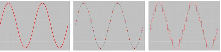
The history of optimal vector quantization theory goes back to the 1950’s in the Bell laboratories where researches were carried out to optimize signal transmission by appropriate discretization procedures. Two kinds of “stationary” signal can be naturally considered: either a deterministic – more or less periodic – signal, denoted by (xt)t≥0, or a stochastic signal, denoted by (Xt)t≥0, considered under its stationary regime and supposed to be
ergodic. In both cases, these signals share an averaging property as will be seen further on. Vector quantization can be briefly introduced as follows.
∗The author thanks B. Jourdain and the referee for their careful reading of the manuscript and S. Graf for fruitful comments
on source coding. All errors are mine.
1Laboratoire de Probabilit´es et Mod`eles al´eatoires, UMR 7599, UPMC, case 188, 4, pl. Jussieu, F-75252 Paris Cedex 5, France.
E-mail: [email protected]
Figure 1. Quantization of a scalar (periodic) signal (B. Wilbertz)
c
EDP Sciences, SMAI 2015
Let Γ ={x1, . . . , xN}be a subset ofR
d (d≥1) of size (at most)N ≥1, called aquantization gridor simply a quantizerat level N if Γ has exactly cardinalityN i.e. if theelementary quantizers xi are pairwise distinct. Whend= 1 the numbering of the elementary quantizersxi isa priorimade consistent with the natural order on the real line so thati7→xi is non-decreasing.
In what follows, except specific mention,|.|will denote the canonical Euclidean norm onRd(although many of the stated results remain true or admit variants for more general norms).
A Γ-valuedquantization function(also calledquantizer) is simply a Borel functionq:Rd→Γ. A naive idea is to transmit at timet the stochastic signalq(Xt) instead ofXtitself inducing a resulting pointwise error
|Xt−q(Xt)|.
One proceeds likewise for a deterministic signal with a resulting error|xt−q(xt)|.
BDeterministic signal: Letp∈(0,+∞). Assume that the empirical measure 1 t
Z t
0
δx(s)dsweakly converges as
t→+∞toward a distributionµon (Rd,Bor(Rd)) such that Z
Rd
|ξ|pµ(dξ)<+∞. If the quantization function
qisµ-a.s. continuous and,e.g., lim sup t→+∞
1 t
Z t
0
|x(s)|rds <+∞for some r > p, then
lim t→+∞
1
t Z t
0
|x(s)−q(x(s))|pds 1p
= Z
Rd
|ξ−q(ξ)|pµ(dξ) 1p
=kξ−q(ξ)kLp(µ)<+∞.
BStationary ergodic stochastic signal: We consider againp∈(0,+∞). Assume the process (Xt)t≥0is stationary.
Then, Xt has the same marginal distribution, say µ, for everyt∈R+. Moreover, ifE|Xt|p= R
Rd|ξ|
pµ(dξ)< +∞, then
kXt−q(Xt)kLp(P)=kX0−q(X0)kLp(P)=kξ−q(ξ)kLp(µ)<+∞. Moreover, if the process (Xt)t≥0is ergodic, ergodic pointwise Birkhoff’s Theorem ensures that
P-a.s. lim t→+∞
1
t Z t
0
|Xs−q(Xs)|pds p1
=kξ−q(ξ)kLp(µ)<+∞.
At this stage, several questions arise to optimize the transmission. Based on what precedes, we will mainly adopt from now on thestatic point of view of anRd-valued random vectorX, defined on a probability space (Ω,A,P), with distribution µ. It corresponds to the value of Xt at any time t or to the asymptotic behavior of the signal (x(t))t≥0. More general situations of quantization or coding can be investigated in Information
Theory which take into account the dynamics of the (ergodic) process leading to the most general Shannon’s source coding theorem. For these deeper aspects from Information Theory, we refer to the general distortion theory as analyzed by large deviation methods in [23] and the references therein.
Question 1How to optimally choose the Γ-valued quantization function q (Geometric optimization)?
It is clear that, whatever the quantization functionq:Rd→Γ is, one has
|ξ−q(ξ)| ≥dist(ξ,Γ)
where dist(ξ, A) = infa∈A|ξ−a| denotes the distance of ξ to the set A ⊂ Rd (with respect to the current norm). One easily checks that equality holds in the above inequality if and only ifqis a Borel nearest neighbour projectioni.e. q=πΓ defined for everyξ∈Rdby
πΓ(ξ) = N X
i=1
where theN-tuple of subsets Ci(Γ)
1≤i≤N is a Borel partition of (R d,Bor(
Rd)) satisfying
∀i= 1, . . . , N, Ci(Γ)⊂nξ∈Rd : |ξ−xi|= min
1≤j≤N|ξ−xj| o
.
Such a partition ofRd is called a Voronoi partition(or sometimestessellation) induced by Γ. When the norm |.| is Euclidean, the closuresCi(Γ) of the cells are non-empty polyhedral closed convex sets (intersection of finitely many half-spaces defined by median hyperplanes of the couples of points (xi, xj), i 6=j). One easily shows that
n
ξ∈Rd : |ξ−xi|< min
1≤j≤N, j6=i|ξ−xj| o
⊂Ci◦ (Γ)⊂Ci(Γ)⊂nξ∈Rd : |ξ−xi|= min
1≤j≤N|ξ−xj| o
.
The inclusions at both ends of the inclusion chain can be replaced by equalitiesin an Euclidean framework. Then, for a given (static) random vector having values inRd, one defines aVoronoi Γ-quantizationof X by Γ as
b
XΓ=πΓ(X).
Remark. For more developments on the non-Euclidean framework, like e.g.the `r-norms defined by |ξ|r = |ξ1|r+· · ·+|ξd|r1r
, r∈[1,+∞), or |ξ|∞= max1≤j≤d|ξj|,ξ= (ξ1, . . . , ξd)∈Rd, we refer to [33], Chapter 1.
This leads us to define for everyp∈(0,+∞) theLp-mean quantization error induced by a grid Γ as
ep(Γ, X) =
X−πΓ(X)Lp( P)=
dist(X,Γ)Lp( P)=
min
1≤i≤N|X−xi| Lp(
P) (1.1)
= min
1≤i≤N|ξ−xi| Lp(µ)=
Z
Rd
min
1≤i≤N|ξ−xi| pµ(dξ)
1p
. (1.2)
Note that, from a computational point of view, the computation ofπΓ(ξ) is very demanding when the sizeN is large since it amounts to a nearest neighbour search. We will come back to that point further on in Section3
devoted to numerical aspects of (optimal) quantization grid computation.
Question 2How to choose Γin order to improve the transmission?
The underlying idea is to try selecting (or designing) a grid Γ with size at most N which optimally “fits” to the distributionµof X, with in mind an approximation in theLp-sense whenX∈Lp
Rd(P). To this end, we
introduce theLp-distortion function.
Definition 1.1. Letp∈(0,+∞)andX∈Lp
Rd(P). TheR+-valued function Gp,N defined on (R
d)N by
Gp,N : (x1, . . . , xN)7−→E
min
1≤i≤N|X−xi| p=e
p(Γ, X)p=
dist(X,Γ) p Lp(P)
is called theLp-distortion function.
It is clear that, if we define the optimalLp-mean quantization problem by
ep,N(X) = inf
Γ,card(Γ)≤Nep(Γ, X) (1.3)
where card(Γ) denotes the cardinality of the grid Γ⊂Rd, then
ep,N(X) = inf
Note that, in fact, ep,N(X) only depends on the distribution µ of X. So we will occasionally write ep,N(µ) instead ofep,N(X). This follows from the easy remark that a grid Γ with less thanN elements can always be represented by anN-tuple in which each element of the grid appears as a component at least once.
Proposition 1.1. Let p∈(0,+∞). Assume that X∈ Lp
Rd(P)i.e.
Z
Rd
|ξ|pµ(dξ)<+∞ so that the distortion
function Gp,N is finite everywhere on (Rd)N.
(a)The distortion function Gp,N attains a minimum at anN-tuplex(N,p)= (x1(N,p), . . . , x(NN,p)).
(b) If card supp(µ)
≥N, then the corresponding grid Γ(N,p) =
x(1N,p), . . . , x(N,p)
N has full size N and for
every Voronoi partition Ci(Γ(N))
1≤i≤N of R
d induced byΓ(N),
P(X∈Ci(Γ(N))>0. (c) The sequenceN 7→ep,N(X)(strictly) decreases as long asN ≤cardsupp(µ)|and
lim
N ep,N(X) = 0.
The proof of this proposition is postponed to Section2.1. The grid Γ(N,p), the correspondingN-tuplesx(N,p)
(there are N! N-tuples obtained by permutations of the components if the grid has full size N) as well as the (Borel) nearest neighbour projectionsπΓ(N,p) are all calledLp-optimal quantizers.
Of course a crucial question in view of possible applications is to compute suchLp-optimal quantizersat level N, especially in higher dimension.
Whend= 1 and µ=U([0,1]), then, for anyp∈(0,+∞), themid-point grid Γ(N,p)=2i−1
2N , i= 1, . . . , N is the unique optimalLp-quantizer at levelN. The attached weights are all equal tow(p,N)
i =
1
N,i= 1, . . . , N, and the resulting optimalLp-quantization error is given for every N ≥1 by
ep,N U([0,1])
= 1
2(1 +p)1/pN. (1.4)
More generally the question of therate of decayofep,N(X) is the central question of optimal vector quanti-zation theory. It will be investigated further on in Section2.3.
1.2.
Application to signal transmission (source coding)
As mentioned in the introduction, this application of (optimal) quantization goes back to the very origin of quantization theory in the 1950’s. Imagine one has access to an Lp-optimal quantization grid, say for p= 2 (quadratic case in an Euclidean setting). For convenience, we assume that Γ = {x1, . . . , xN} is a grid (possibly optimal) such that P X∈S1≤i≤N∂Ci(Γ)
=µ S
1≤i≤N∂Ci(Γ)
= 0 e.g.becauseµassigns no mass to hyperplanes.
What is the information “contained” inXbΓ=πΓ(X)? Or equivalently, in probabilistic terms, what are the
characteristicsof the distribution ofXbΓ? (1) Its state space Γ ={x1, . . . , xN},
(2) Its “companion” weightswi=wi(Γ)=P(XbΓ=xi) =P(X∈Ci(Γ)) =µ(Ci(Γ)),i= 1, . . . , N.
IfX is a random vector with a known simulatable distributionµ, one can pre-compute these weightswiwith an arbitrary accuracy by a large scale Monte Carlo simulation since, owing to the Strong Law of large Numbers,
wi=P-a.s. lim M→+∞
cardn1≤m≤M : |Xm−xi|<minj6=i|Xm−xj o
M , i= 1, . . . , M,
where (Xm)m≥1 is a sequence of i.i.d. random vectors with distributionµ. In case of a not too large dataset (a
1.2.1. Coding the (quantized) signal
Let Γ ={x1. . . , xN} ⊂R
d be a grid of sizeN, possibly sub-optimal at this stage, and let P(Γ) be the set of distributions whose support is exactly Γ. In order to transmit a Γ-valued signal from a senderA to a receiver B, A will transmit acodeword Ci =C(xi)representative of xi instead of (an accurate enough approximation of) xi itself. For simplicity we will assume that the coding function C maps Γ into the set {0,1}(N) of finite
{0,1}-valued sequences. This means that we adopt a dyadic coding procedures. The set {0,1} is called a 2-alphabet (1). Our first request on the function C is identifiability i.e. that B can always recover xi from Ci or equivalently that C is injective. To design the codewords (Ci)1≤i≤N, one aims at minimizing the mean
transmission cost κ, also known as the mean lengthof the message. This is in fact a very old problem which goes back to the origins of Information Theory introduced by Claude Shannon in [71].
Let us focus for a while on this coding problem. The mean transmission cost κ(N) for a grid of size N is clearly defined by
κ(N) = N X
i=1
wi×length(Ci).
A first (not so) naive idea is to re-index the points xi by a permutationσ so thati7→wσ(i) is non-increasing.
Without loss of generality, we may assume from now on that σ is identity (though, for one-dimensional dis-tributions, it is not consistent in general with the natural order of the points xi on the real line). Then, it is intuitive (but in fact not mandatory) to devise the coding functionCso thati7→length(Ci) is non-decreasing since, doing so, the more often a code is transmitted, the shorter it will be. In case of equality, like for the uniform distribution over Γ, assignment conventions have to be made.
The naive approach is to simply codexi through the regular dyadic expression ¯i2ofiwhich needs 1 +blog 2ic
digits (wherebξcdenotes the lower integer part ofξ∈R). This yields
κ(N) = N X
i=1
wi 1 +blog2ic = 1 +
N X
i=1
wiblog2ic ≤1 +blog2Nc.
The transmission relies on the fact that bothA andB share thecodebooki.e.a one-to-one correspondence
xi←→¯i 2
. (1.5)
A toy example. Imagine that, to transmit a uniformly distributed signal over the unit interval [0,1], we first
optimally quantize it using the mid-point grid Γ(N)=n2i−1
2N , i= 1, . . . , N o
. This is equivalent to transmit a
uniformly distributed signal over{1, . . . , N}thanks to the codebook so that, as far as transmission is concerned, the grid Γ(N) itself plays no role. The resulting mean transmission costκ(N) is equal to
κ(N) = 1 + 1 N
N X
i=1
blog2ic ∼log2 N/e
as N →+∞.
To be more precise, once noted that the dyadic entropy H2 µˆU nifN of the uniform distribution ˆµU nifN over
{1, . . . , N}(or equivalently on Γ(N)) is equal to log
2N, we can show that
c− = lim inf N
κ(N)−H2 µˆU nifN
≤lim sup N
κ(N)−H2 µˆU nifN )
=c+
wherec−≈ −2,8792 andc+≈ −0.9139.
1.2.2. Instantaneous coding.
However, this approach is definitely too naive. In practice, A does not send one isolated codeword but a sequence of codewords. Such a coding is not satisfactory, mainly because it is not self-punctuated. To be decodable, an extra symbol (space, comma, etc) is needed to isolate the codewords. Doing so amounts to adding one symbol to the alphabet (with a special status since it cannot be repeated, like the large space in Morse coding). But this lowers the global performance of the coding system since it inducesde factoswitching from a 2-alphabet to a 3-alphabet coding function C, the third symbol having moreover a lower status of “under-symbol”. To overcome this problem, the idea, again due to Shannon in his seminal 1948 paper [71], is to devise
self-punctuated codes. This relies on two conditions. First we ask the coding process to beuniquely decodable
in the sense that the concatenation of codewords C(x1)· · ·C(xN) uniquely characterizes the concatenation x1· · ·xN. The additional condition which defines an instantaneous coding system is that a codeword can never be the prefix of another or, equivalently, no codeword can be obtained as the concatenation of another codeword and further symbols of the alphabet (here 0 and 1 digits). One easily checks that an instantaneous coding procedure is always self-punctuated.
Unfortunately, it is also straightforward to check that the naive dyadic coding (1.5) formerly mentioned which consists in writing in base 2 every indexiis notan instantaneous coding system since,e.g., ¯22= 10 and ¯
52= 101.
Let us illustrate on a simple example how an instantaneous coding procedure look. We consider the following coding procedure of the set of indices{1,2,3,4}:
C(1) = 0, C(2) = 10, C(3) = 110, C(4) = 111.
Such a code is uniquely decodable (e.g.0110111100110 can be uniquely decoded as the string 134213). Further-more it is clearly instantaneous (thus 010111110010 can be parsed on line as 0,10,111,110,10 i.e. the string 12432).
If we consider the uniform distribution ˆµU nif
4 over{1,2,3,4}, the resulting mean transmission cost is equal to κ µˆU nif
4
:= 1
4(1 + 2 + 3 + 3) = 9
4 whereas the naive dyadic coding of the indices seemingly yields
8 4 = 2.
However, theimplementableversion of this naive dyadic coding (1.5),i.e.including an extra symbol like “,”, has a mean length equal to 3> 9
4. This can be up to 30% more symbol consuming than the above instantaneous
code!
Now, let us consider a general distribution µˆN exactly supported by{1, . . . , N} (or equivalently by a grid ΓN of sizeN) anda priori not uniform. Assume we have access to the distribution ˆµitself i.e.to the weights wi= ˆµN {i}
. We define the dyadic entropyH2(ˆµ) of ˆµby
H2(ˆµ) =−
N X
i=1
wilog2wi.
Then, the following classical theorem from Information Theory holds (see [20], Chapter 5, Theorem 5.3.1 and Section 5.4).
Theorem 1.1. For any instantaneous dyadic coding procedureC:{1, . . . , N} → {0,1}(N)of the distributionµˆ, its mean transmission cost κµˆ(N)satisfies
κ(ˆµN)≥H2(ˆµN). (1.6)
Furthermore, there exists (at least) one instantaneous coding procedure such that
For a proof of this result based on Kraft’s inequality, which is too far from the scope of this paper, we refer to [20]. Furthermore, when a sequence (Yn)n≥0of{1, . . . , N}-valued signals to be transmitted is stationary with
marginal invariant distribution ˆµN and ergodic, it is possible by aggregating nof them to show (with obvious notations, see again [20]) that
κ(Y1, . . . , Yn)→H2(ˆµ)a.s. asn→+∞. (1.8)
Examples. (a)The Huffman code: It was the first optimal instantaneous code – devised in Huffman’s PhD thesis (see also [38]). Its length sequence (`∗
i)1≤i≤N can be obtained as the solution to the integer optimization problem (`i denotes the length of a code Ci):
`∗= argmin P2−`i≤1
X wi`i
so thatH2(ˆµN)≤κHuf(ˆµN) = Pw
i`∗i ≤H2(ˆµN) + 1. For an explicit construction of the Huffman code – and not only of its length sequence!) – we refer again to [20], Chapter 5. Let us simply mention that the codes are obtained by the concatenation of labels given to the edges, say 1 for “right” edges, 0 for “left edges” starting from the root, of successive trees built from the increasing monotony of the weights wi. The successive trees are obtained by summing up the lower probabilities, starting from weN−1 := wN +wN−1, with appropriate
conventions in case of equality like with uniform distributions.
(b)The Shannon coding (see exercise 5.28 in [20]): Still assume that the weights of the distribution ˆµN satisfy 0< wN ≤ · · · ≤w1<1. LetF
ˆ
µN denote thestrict-cumulative distribution function of ˆµ
N defined by
FµˆN i =
X
j<i wj.
Set
`i=d−log2wie and Ci=b2`iFµˆ
i c, i= 1, . . . , N,
wheredξedenotes the upper integer part of the real numberξ. Elementary computations show that Shannon’s code is instantaneous and that its mean transmission cost κShanS(ˆµN) also satisfies
H2(ˆµN)≤κShanS(ˆµN)< H2(ˆµN) + 1.
1.2.3. Global error induced by the transmission of a quantized signal
Let us bring back quantization into the game by considering a continuous signal which needs to be quantized in order to reduce its transmission cost. Let us briefly compare from a quantitative viewpoint two modes of transmission for a signal.
BDirect transmission. Let (Xt)t≥0 be a stochastic stationary signal with marginal distribution µ defined on
a probability space (Ω,A,P) and Γ ={x1, . . . , xN}. To transmit the Γ-quantizationXbΓ of the random signal X =Xt0 at timet0, the resulting quadratic mean quantization error is equal to
X−XbΓ
L2(P)+ 2 −r=e
2(Γ, µ) + 2−r
where 2−r is the dyadic transmission accuracy of any of the elementary quantizersx
i. In fact this corresponds to a fixed transmission costκ=r+ 1i.e. thenumber of dyadic digitsused to transmit these values. Common values for rlie between 10 and 20 (having in mind that 2−10= 1
1024 ≈10
B Signal transmission using the codebook. If the receiver B uses the codebook (Ci ←→ xi)1≤i≤N for the decoding phase (2), the resulting mean quadratic transmission error will be equal to
X−XbΓ
L2(P)=e2(Γ, µ)
whereas the mean unitary transmission cost is κµ(Nˆ ) where ˆµ is the distribution of the quantized signalXbΓ. In this second case, there is a connection between the transmission error and the transmission cost that will be made more precise in Section2.3when the grid Γ isL2-optimal at levelN forµ.
However, in the very simple case of the uniform distributionU([0,1]) over the unit interval, we can establish a direct relation between quadratic mean transmission error and mean transmission cost κ when both the quantization and the instantaneous coding are optimal. The optimal quadratic quantization of U([0,1]) is the uniform distribution ˆµU nif
N over the N-mid-point whose dyadic entropy is exactly H2(ˆµ U nif
N ) = log2N. Plugging this equality in (1.7) yieldsκµˆN ≤log2(N). In turn, plugging this inequality in the quantization error
bound (1.4) yields thatthe lowest achievable mean transmission error, for a prescribed mean transmission cost κ, approximately satisfies
2−(κ+1) √
3 ≤L
2-Mean transmission error(κ)≤2√−κ
3. A less sharp (reverse) formulation is
−log2 Transmission error(κ)
∼κ as κ→+∞.
This result appears as the most elementary version of Shannon’s source coding theorem, here in one dimension. Its extension to more general distributionsµonRd will be possible, once stated the sharp convergence rate of theL2-optimal mean quantization error for general distributions onRd in Section2.3(Zador’s Theorem).
We focused in the above lines on a static random signal presentation but the adaptation to a stationary process or a quasi-periodic signal, as defined above in terms of weak convergence of its time empirical measure, is straightforward. In particular for stationary ergodic signal one may take advantage of the improvement provided by (1.8), using n-aggregates of the signal, to reduce the range of the two-sided inequality (1.6)-(1.7) in Theorem1.1.
1.3.
What else is quantization for?
1.3.1. Data mining, clustering, automatic classification
Let (ξk)1≤k≤nbe anRd-valued dataset and letµbe the uniform distribution over this dataset – the empirical measure of the dataset – defined by
µ= 1 n
n X
k=1
δξk (1.9)
whereδadenotes the Dirac mass ata∈Rd. In such a framework,nis usually large, say 106or more, and optimal quantization can be viewed as a model for clusteringi.e.the design of a set ofN prototypesof the dataset, with N n, obtained as a solution to the mean quadratic (or more generally Lp-) optimal quantization at level N ≥1 of the distributionµ(p∈(0,+∞) being fixed). This reads as theLp-minimization problem
min
(x1,...,xN)∈(Rd)N 1 n
n X
k=1
min
1≤i≤N|ξk−xi| p.
2The senderAonly needs a codebook to discriminate the elementary quantizersx
ii.e.a codebook where allxiare known with a fixed length`1(dyadic) bits in its dyadic representation. The receiverBmay need arbitrary accurate values for the elementary
The existence of such an optimalN-quantization grid Γ(N,p)of prototypes follows from the above Proposition1.1.
Such a distribution does assign mass to hyperplanes and in particular to the boundaries of polyhedral Voronoi cells. However, owing to Theorems 4.1 and 4.2 in [33] (p.38), we know that the boundaries of the Voronoi cells induced by an optimal grid Γ(N,p)are alwaysµ-negligible.
Once an optimized grid ofN prototypes has been computed (see Section3devoted to the algorithmic aspects), it can be used to produce an automatic classification of the dataset by making up “clusters” of points of the dataset following the nearest neighbour rule among the prototypes. Formulated equivalently, one defines theN clusters as the “trace” of the dataset on theN Voronoi cellsCi(Γ(N,p)),i= 1, . . . , N.
From a mathematical point of view, investigations on this topic are carried out be replacing the deterministic dataset (ξk)1≤k≤n by a sequence of i.i.d. random vectors (Xk)k≥0 defined on a probability space (Ω,A,P) with distributionµ. The quantities of interest become, in short, the sequence of optimization problems induced by the random empirical measuresµn(ω, dξ) = n1
Pn
k=1δXk(ω)(dξ),ω∈Ω. This has given rise to a huge literature in Statistics and has known a kind of renewal with the emergence of clustering methods in the “Big Data” world, see [10]. We consider, for everyω∈Ω, the optimization problem
min
(Rd)N "
1 n
n X
k=1
min
1≤i≤N|Xk(ω)−xi| p=
Z
Rd
min
1≤i≤N|ξ−xi|
pµn(ω, dξ) #
. (1.10)
The main connection with optimal quantization is the following. assume that µ(B(0; 1)) = 1. For every ω∈Ω, there exists (at least) an optimalN-tuplex(N)(ω, n) for the above problem which satisfies
E
e2 x(N)(ω, n), µ
−e2,N(µ)≤Cmin
r
N d n ,
s d N1−2
dlogn n
where C > 0 is a positive universal real constant. For other results, we also refer to [34] devoted to the quantization rate of empirical measures.
1.3.2. From Numerical integration (I) . . .
Another way to take advantage of optimal quantization emerged in the 1990’s (see [55]). As we know, for a sequence (Γ(N,p))N≥1ofLp-optimal grids of sizeN withN →+∞, we have
kX−XbΓ (N,p)
kLp(P)=ep,N(X)→0
i.e. XbΓ (N,p)
→ X in Lp as N → +∞ (hence in distribution). It can be shown (see [22]) that, in fact, this convergence also holds in an a.s. sense although we will make little use of this feature in what follows. In particular, if a function F : Rd →R is bounded and continuous, then EF(XbΓ
(N,p)
) →EF(X) as N →+∞. On the other hand, using the characteristics (xi(N), wi(N))1≤i≤N of the distribution of XbΓ
(N,p)
, we derive a very simple weightedcubature formula
EF XbΓ (N,p)
= N X
i=1
w(iN)F x(iN)
. (1.11)
WhenF has more regularity and is possibly not bounded, precise error bounds for this quantization based cubature formula can also be established, as we will see now.
First order error bound for the quantization based cubature formula. Assume F is locallyα-H¨older continuous in the sense that there exists α∈(0,1],β≥0, and a real constant [F]α,β such that
∀x, y∈Rd, |F(x)−F(y)| ≤ [F]
Let Γ⊂Rd be a quantization grid. Then, for every conjugate H¨older exponents (p, q)∈[1,+∞],
EF(X)−EF(XbΓ)
≤ [F]α,βE
|X−XbΓ|α 1 +|X|β+|XbΓ|β)
≤ [F]α,βkX−XbΓkαLαp(P)
1 +kXkβLβq(P)+kXbΓk β Lβq(P)
.
In particular, ifp= α1, one gets
EF(X)−EF(XbΓ)
≤[F]α,βkX−XbΓkα1
1 +kXkβ L
β 1−α(P)
+kXbΓk β
L β 1−α(P)
(1.12)
with the conventionk.k0
L β 1−1(P)
= 1. IfF isα-H¨older continuous with Lipschitz coefficient [F]α=13[F]1,0, then
EF(X)−EF(XbΓ)
≤F]αkX−XbΓkαLα(P). (1.13)
From the cubature formula (1.13) and using that bounded H¨older functions characterize the weak convergence of probability measures, we derive the following corollary aboutLp-optimal quantizers (by consideringα=p∧1).
Corollary 1.1. Let X∈Lp
Rd(P),p∈(0,+∞), with distribution µ. Let (Γ
(N))
N≥1 be a sequence of quantizers, withΓ(N)of sizeN, satisfyinge
p(Γ(N), µ)→0asN →+∞. LetµˆN denote the distribution of the quantization b
XΓ(N). Then
ˆ µN =
N X
i=1
µ Ci(Γ(N)) δx(N)
i
(w)
−→µ as N →+∞ (1.14)
whereΓ(N)={x(N) 1 , . . . , x
(N)
N } and
(w)
−→ denotes the weak convergence of distributions.
1.3.3. . . . to Numerical Probability (conditional expectation)
One of the main problem investigated in the past twenty years in Numerical Probability has been the
numerical computation of conditional expectations, mostly motivated by problems arising in finance for the pricing of derivative products of American style or more generally known as “callable”. It is also a challenging problem for the implementation of numerical schemes for Backward Stochastic Differential Equations (see [2,3]), Stochastic PDEs (see [32]), for non-linear filtering [57,68] or Stochastic Control Problems (see [13,14,58]). Further references are available in the survey paper [62] devoted to applications of optimal vector quantization to Numerical Probability. The specificity of these problems in the probabilistic world is that, whatever the selected method is, it suffer in some way or another from the curse of dimensionality. Optimal quantization trees (introduced in [2]) is one of the numerical methods designed to cope with this problem (with regression and Monte Carlo-Malliavin method, see [46], [28]). The precise connection between vector quantization and conditional expectation computation can be summed up in the proposition below.
We consider a couple of random vectors (X, Y) : (Ω,A,P) → Rd ×Rq and the regular version Q of the conditional distribution operator of X given Y, defined on every bounded or non-negative Borel functionf : Rd→R, by
Qf(y) =E f(X)|Y =y.
Then, Qf is a Borel function on Rd. We define the Lipschitz ratio of a function f : Rd → R by [f]Lip =
supx6=y|f(y|x−y|)−f(x)| ≤ +∞. We make the following Lipschitz continuity propagation assumption on Q: there exists [Q]Lip∈R+ such that
Proposition 1.2. Assume that the conditional distribution operatorQofX givenY satisfies the above Lipschitz continuity propagation property (1.15). Let ΓX ⊂ Rd and ΓY ⊂ Rq be two quantization grids of X and Y
respectively.
(a) Quadratic case. Assume X, Y ∈ L2(
P). Let f : Rd → R be a Lipschitz continuous function and let g:Rd→
Rbe a Borel function with linear growth. Then
E f(X)|Y
−E g(XbΓX)|YbΓY
2
L2(P)≤[Qf]
2 Lip
Y −YbΓY
2
L2
Rq(P)
+f(X)−g(XbΓX)
2
L2(P)
so that ifg=f,
E f(X)|Y
−E f(XbΓX)|YbΓY
2
L2
Rq(P)
≤[Qf]2LipY −YbΓY
2
L2(P)+ [f]
2 Lip
X−XbΓX
2
L2(P).
(b) Lp-case. Assume X,Y∈Lp(
P),p∈[1,+∞)and letf andg be like in(a). Then
E f(X)|Y
−E g(XbΓX)|YbΓY
Lp
Rq(P)
≤(2−δp,2)[Qf]Lip
Y −YbΓY Lp(P)+
f(X)−g(XbΓX) Lp(P)
whereδp,p0 denotes the Kronecker symbol. In particular, if g=f, one has
E f(X)|Y
−E f(XbΓX)|YbΓY
Lp(P)≤(2−δp,2)[Qf]Lip
Y −YbΓY Lp
Rq(P)
+ [f]Lip
X−XbΓX Lp(P).
Proof. (a) We decomposeE f(X)|Y
−E f(XbΓX)|YbΓY
into two (L2(
P)-orthogonal) terms
E f(X)|Y−E f(XbΓX)|YbΓY
= E f(X)|Y
−E E(f(X)|Y)|YbΓY
| {z }
(1)
+E E(f(X)|Y)|YbΓY
−E g(XbΓX)|YbΓY
| {z }
(2)
.
To check the announcedL2(
P)-orthogonality, we note that (2) isσ(YbΓY)-measurable; hence, the character-ization of conditional expectation given YbΓY impliesE(1)×(2) = 0. On the other hand, the very definition of conditional expectation given YbΓY as the best approximation in L2
Rq(P) by a square integrable σ(Yb
ΓY
)-measurable random vector implies in turn
E(1)2 = E Qf(Y)−E(Qf(Y)|YbΓY) 2
≤E Qf(Y)−Qf(YbΓY) 2
≤ [Qf]2LipY −YbΓY
2
L2(P).
On the other hand, using that YbΓY is σ(Y)-measurable, we first derive from the chain rule for conditional expectation that
(2) =E f(X)|YbΓY
−E g(XbΓX)|YbΓY
=E f(X)−g(XbΓX)|YbΓY
.
Using now that conditional expectation is anL2-contraction, we deduce that
E(2)2≤ kf(X)−g(Xb
ΓX)k2
L2(P)≤ kf(X)−g(Xb
ΓX)k2 L2
Rq(P)
.
(b) We start from the classical Minkowski Inequality
E f(X)|Y
−E g(XbΓX)|YbΓY
Lp(P) ≤
Qf(Y)−E(Qf(Y)|YbΓY) Lp(P)
+E f(X)|YbΓY
−E g(XbΓX)|YbΓY
Lp(P)
where we used like in (a) thatE Qf(Y)|YbΓY
=E f(Y)|YbΓY
. Now, still owing to Minkowski’s Inequality,
Qf(Y)−E(Qf(Y)|YbΓY) Lp(P)≤
Qf(Y)−Qf(bYΓY) Lp(P)+
E Qf(bYΓY)−Qf(Y)|YbΓY
Lp(P)
so that
Qf(Y)−E(Qf(Y)|YbΓY)
Lp(P) ≤ 2
Qf(Y)−Qf(YbΓY) Lp(P)
≤ 2[Qf]Lip
Y −YbΓY Lp
Rq(P)
.
Note that whenp= 2 the above coefficient 2 can be cancelled using again, like in (a), that conditional expectation givenYbΓY is the bestapproximatorinL2(P) byσ(YbΓY)-measurable square integrable random vectors. On the other hand,
E f(X)|YbΓY
−E g(XbΓX)|YbΓY
Lp(P) ≤
f(X)−g(XbΓX) Lp(P).
The case g=f follows immediately. This completes the proof.
To conclude this section, we make the connection between these cubature formulas and theL1-Wasserstein distanceW1 defined by
W1(µ, ν) = inf
n
EP|X−Y|, X, Y : (Ω,A,P)→R
d, X d
=µ, Y =d νo
where= denotes the identity in distribution.d
Proposition 1.3. Let X∈Lp
Rd(P),p∈(0,1], with distributionµand letΓ ={x1, . . . , xN}. (a)For every p∈(0,1],kX−XbΓk
p
Lp(P)= sup
[F]p≤1
|EF(X)−EF XbΓ
where [F]p = supx6=y
|F(x)−F(y)|
|x−y|p denotes
the p-H¨older coefficient of the functionF :Rd→R.
(b) IfPN denotes the set of probability measures with a support having at most N points inRd, then
W1(µ,PN) =e1,N(µ).
Proof. (a) The inequality sup
[F]p≤1
EF(X)−EF XbΓ
≤ kX−XbΓk p
Lp(P)is straightforward by settingα=pand β = 0 in (1.12) and noting that [F]p =13[F]p,0. The equality follows by noting that the functionFp defined for
every ξ∈Rd byFp(ξ) = min1≤i≤N|ξ−xi|p isp-H¨older with [Fp]p= 1. (b) LetX : (Ω,A,P)→Rd with distribution
PX =µ. It is clear, as already seen, that ifY : (Ω,A,P)→R d is
such that ΓY =Y(Ω) has at mostN values, then|X−Y| ≥dist(X,ΓY) =|X−XbΓY|so thatkX−XbΓYk1≤
E|X−Y|. As a consequencee1,N(µ)≤ W1(µ,PN). Conversely, it follows from the definition ofe1,N(µ) in (1.3) thate1,N(µ)≥ W1(µ,PN) since it is defined as an infimum overlessrandom vectors, namely those of the form Y =q(X) of X whereq:Rd →
1.4.
Application to Numerical Analysis
1.4.1. Representation and numerical approximation of the solution of parabolicP DE, Feynman-Kac’s formula
Let b : [0, T]×Rd →Rd and a : [0, T]×Rd → S+(d,R) be two continuous functions with at most linear and quadratic growth in x, uniformly with respect tot∈[0, T], respectively (S+(d,
R) denotes the set ofd×d symmetric non-negative matrices). Let f :Rd →
Rbe a Borel function with polynomial growth. We want to solve numerically the following parabolic partial differential equation (P DE), either by a Monte Carlo simulation or by a quadrature formula
∂u
∂t +Lu= 0, u(T, .) =f (1.16) where, denoting by (.|.) the canonical inner product onRd,
Lu= (b|∇u) +1 2Tr(a∇
2u). (1.17)
BStep 1 (Feynman-Kac’s representation formula). This fundamental connection between diffusion process and (parabolic) PDEs is summed up in the following theorem.
Theorem 1.2(Feynman-Kac’s representation formula). Assume (for simplicity) that the functionsbandaare such that the above PDE (1.17)has a unique C1,2([0, T]×
Rd)solution uwhose gradient∇xu has polynomial
growth in x, uniformly in t∈[0, T]. Let σ:Rd → M(d, q,R)(3) such that a=σσ∗ (where ∗ stands for matrix
transposition). Assume that b and σ are continuous on [0, T]×Rd and, at least, Lipschitz continuous in x,
uniformly in t∈[0, T].
(a)Then the function uadmits the following representation as an expectation:
∀x∈Rd, ∀t∈[0, T], u(t, x) =Ef(XTt,x)
where(Xx,t
s )s∈[t,T] denotes the unique solution to the Stochastic Differential Equation (SDE)
dXst,x=b(s, Xst,x)ds+σ(s, Xst,x)dWs, X t,x
t =x, s∈[t, T], (1.18)
starting from x∈ Rd at time t∈[0, T] and defined on [t, T], where W is a q-dimensional standard Brownian
motion defined on a probability space (Ω,A,P).
Owing to the Markov property, an alternative formulation is given by
∀t∈[0, T], E f(XT)|Xt
=u(t, Xt) a.s.
for any solution(Xt)t∈[0,T] of the aboveSDE defined over the whole interval[0, T] starting at a finite random vectorX0 independent ofW. In particularu(t, x) =E f(XT)|Xt=x
(in the sense that it is a regular version of the conditional expectation as xvaries).
(b) Time homogeneous diffusion coefficients: Ifb(t, x) =b(x) andσ(t, x) =σ(x) (no dependence ofb andσ in
t), then the representation can be written
∀x∈Rd, ∀t∈[0, T], u(t, x) =Ef(XT0,x−t). (1.19)
Proof. (a) Itˆo’s formula applied to the functionuand the process (s, Xt,x
s )s∈[t,T] betweentandT yields
u(T, Xt,x
T ) =u(t, x) + Z T
t ∂u
∂t +Lu
(s, Xst,x)
| {z }
=0
ds+ Z T
t
∇xu(s, Xst,x)|σ(s, X t,x s )dWs
.
The integral in “ds” is zero since usatisfies the parabolic PDE (1.16) and one easily establishes that the local martingale null at 0 defined by the Brownian stochastic integral is a true martingale, null at 0, owing to the growth control assumption made on∇xu. Then, one gets
Eu(T, XTt,x) =u(t, x).
(b) One writes Itˆo’s formula between 0 andT−ttou(T−t, Xt0,x) and proceeds as above.
Remark. In the time homogeneous case, one can proceed by verification. Under smoothness assumption on b andσ, sayC2 with bounded existing derivatives and H¨older second order partial derivatives, one shows, using
the tangent process of the diffusion, that the functionu(t, x) defined by (1.19) isC1,2in (t, x). Then, the above
claim (b) shows the existence of a solution to the parabolic P DE (1.16).
BStep 2a (Monte Carlo simulation). Assume for the sake of simplicity that we want to compute a numerical approximation of u(0, x) =Ef(X0,x
T )i.e. that t = 0. At this stage, the idea is to replace the diffusion by its
Euler schemewith step Tn, n≥1, starting atx: let tn k =
kT
n ,k = 0, . . . , nbe the uniform mesh of [0, T] with step Tn. It is recursively defined as follows (to alleviate notations, we drop the dependance in 0,x of the Euler scheme):
¯ Xtnn
k+1 = ¯X n tn k + T nb(t n k,X¯
n tn
k) + r
T nσ(t
n k,X¯
n tn
k)U
(n)
k+1, k= 0, . . . , n, X¯
n
0 =x
where (Uk(n))k=1,...,nis an i.i.d. sequence ofN(0;Iq)-distributed random vectors representative of the Brownian incrementsi.e.
Wtn
k−Wtnk−1 = r
T nU
(n)
k , k= 1, . . . , n. As T =tnn, the quantityEf( ¯XTn) is the counterpart of Ef(X
0,x
T ) for the Euler scheme. Assume b and σ are Lipschitz continuous in (t, x) so that the regularity assumption of Theorem1.2is satisfied. Then,
sup n≥1
0max≤k≤n|
¯ Xtnn
k| Lp(P)+
sup
t∈[0,T]
|Xt0,x|
Lp(P)≤κp,b,σ,T 1 +|x|
(1.20)
and, on the other hand, the discrete time Euler schemestronglyconverges toX for the sup norm in everyLp( P) at rateq1
n in the following sense
k=0max,...,n| ¯ Xtnn
k−X
0,x tn
k
Lp(P)≤Cp,b,σ,T r
T
n 1 +|x|
.
As a consequence,Ef( ¯XTn)→Ef(X
0,x
T ) with aO q
1
n
-rate as the stepTn goes to 0 iff is Lipschitz continuous. This latter convergence still holds, without rate, iff is continuous with polynomial growth. It can be obtained under less stringent assumptions on b and σ (continuity in (t, x) and linear growth inxuniformly in t) since then a functional weak convergence holds.
By contrast, if b, σ and f are smooth enough then, the so-called weak error Ef( ¯Xn
T)−Ef(X
0,x
T ) can be investigateddirectlyby more analytic methods. As a result, a (faster)O n1-rate can be established (see [74]). This rate can be extended to bounded Borel functionsf, providedσsatisfies a uniform ellipticity property – or even a hypo-ellipticity assumption “`a la H¨ormander” for a modified Euler scheme – as proved in a celebrated Bally-Talay’s paper (see [7]). This yields
u(0, x) =Ef(XT0,x) =Ef( ¯X n T) +O
1 n
The point of interest at this stage is of course that the expectationEf( ¯Xn
T) can be computed bysimulation since the Euler scheme can be straightforwardly simulated as soon as b and σare computable functions (and X0itself can be simulated). So, we can implement a Monte Carlo simulation to computeEf( ¯XTn)i.e. simulate M i.i.d. copies ( ¯XTn)mm=1,...,M of the above Euler scheme at timeT =tnn and approximateEf( ¯XTn) by the strong Law of Large Numbers
Ef( ¯XTn)≈ 1 M
M X
m=1
f ( ¯Xn T)m
sincea.s.convergence holds asM →+∞. This second error (known as the Monte Carlo or thestatistical error) is of orderO(√1
M) owing to the Central Limit Theorem which provides (asymptotic) confidence intervals for an
a prioriprescribed given confidence level involving the asymptotic variance
Var f( ¯Xn T)
=E f( ¯Xn
T)−Ef( ¯X n T)
2
=Ef( ¯Xn T)
2−
Ef( ¯XTn) 2
.
This variance can be expressed by expectations of functions of ¯XTn, consequently it can be computed on line
as a companion parameter of the original Monte Carlo simulation. By the way, note that one often has Var f( ¯Xn
T)
≈ Var f(XT)), either because f is continuous or because the diffusion is “elliptic enough”, see above. For more details on these elementary aspects of the Monte Carlo method, we refer to classical textbooks devoted Monte Carlo simulation and Numerical Probability (see [43] for a more PDE oriented introduction to Monte Carlo method or [31,56] for more connections with Finance, among many others).
The main asset of this approach is that it is dimension free, in the sense that its complexity grows linearly with the dimensiondof the diffusion of interest, with little influence of the ellipticity of the functiona, at least when the functionf is regular as we just saw.
BStep 2b (Quantization based cubature formula). If one has many computations to carry out with the same operatorL,e.g.for various functionsf, it may be interesting to replace the Monte Carlo simulation by acubature
formula based on an optimal quantization of ¯Xn
T. To perform this quantization, as it will be seen further on in Section3, one can rely on a stochastic optimization procedure which can be viewed as a kind ofcompressed Monte Carlosimulation. In that perspective, one faces now the following chain of approximations
u(0, x) =Ef(X0,x
T )≈Ef( ¯X n T)≈Ef
d¯ Xn T
Γ(N)
where Γ(N)is an optimal (quadratic) quantization grid for the random vector ¯Xn T.
1.5.
Toward automatic meshing.
An alternative to the direct quantization procedure is to consider the grid Γ(N)as a starting point to produce an optimized mesh for the numerical solving of the originalP DE by deterministic schemes like finite element or finite volumes methods, etc. In such an approach, an optimal grid needs to be produced at each discretization timetnk. This approach has been widely investigated by Gunzberger’s group in Florida (USA) (seee.g.[25] and the references therein). More recently, a new concept of quantization (dual quantization, see [64]) has refined this point of view by switching from Voronoi diagrams to a direct approach based on optimized Delaunay triangulations. The resulting grids are better adapted to deterministic numerical analysis methods in medium dimensions.
1.5.1. From optimal stopping theory to variational inequalities
B Discrete time optimal stopping theory in a Markov framework.We consider a standard discrete time Mar-kovian framework: let (Xk)0≤k≤n be anRd-valued (Fk)0≤k≤n-Markov chain defined on the filtered probability space (Ω,A,(Fk)0≤k≤n,P): the chain is (Fk)0≤k≤n-adapted, i.e. Xk isFk-measurable for every k = 0, . . . , n, with transitions
Pk(x, dy) =P Xk+1 ∈dy|Xk=x
so that for every bounded or non-negative Borel functionf :Rd→R,Pkf(x) = Z
Rd
f(y)Pk(x, dy) and
E f(Xk+1)| Fk
=E f(Xk+1)|Xk
=Pk(f)(Xk)a.s.
From now on, we denote byF the filtration (Fk)0≤k≤n. Intuitively,Fk is aσ-field ofAwhich represents the
observable(oravailable)informationat time k. LetZ = (Zk)0≤k≤n be anF-adaptedobstacle/payoff sequence of non-negativeintegrablerandom variables of the form
0≤Zk=fk(Xk)∈L1(Ω,Fk,P), k= 0, . . . , n.
In term of modeling, this can be understood as follows: an agent plays a stochastic game. Each round of the game takes place at timek∈ {0, . . . , n}. The random variableZk represents the reward when leaving the game at timek. The question: “Is there an optimal way to quit the game in order to maximize the gain?”
By “quitting the game”, we mean leaving possibly at arandom timeτ : Ω→ {0, . . . , n}but always honestly i.e. in such a way that, for every`∈ {0, . . . , n}, the event
{τ=`}=
ω∈Ω|τ(ω) =` ∈ F`.
Thus, if the agent adopts this strategyτ, the available information that leads him/her to leave the game at time τ(ω) is the following: if`=τ(ω), for everyA∈ F`, he/she knows whetherω belongs or not toA. In particular the agent has observed the whole path (Xk(ω))0≤k≤τ(ω)since the chain is F-adapted. Such a random variable
is called anF-stopping time. In practice, one can imagine that reasonable strategies will involve or rely on the payoff sequenceZ`)`=f`(X`),`= 0, . . . , n.
Imagine now that this agent enters the game at timek∈ {0, . . . , n}. The aim of the agent is to attain the optimal possible mean gain given the available information at timek, namely
Uk=P-esssupnE Zτ| Fk
, τ : (Ω,A)→ {k, . . . , n},F-stopping timeo (1.21)
with an optimal mean gain given by EUk. The next question is to know whether there is anoptimal stopping
time(or equivalently anoptimal strategy), when starting the game at timek,i.e.a{k, . . . , n}-valuedF-stopping timeτk satisfying
Uk =E Zτk| Fk
.
For more details on this topic we refer to [53] or [42] (Chapter 2) or, more recently, [44].
The sequenceU = (Uk)0≤k≤n is known as the (P,F)-Snell envelopeof the sequence (Zk)0≤k≤n.
From a numerical point of view, we want to compute, or at least approximate, this Snell envelope, especially at time 0, and the related optimal stopping timeτ0(if any).
The first important result of discrete time optimal stopping theory is the following Backward Dynamic Programming Principle (BDP P). Temporarily assume that (Zk)0≤k≤n is an F-adapted general sequence of non-negative integrable random variables.
Proposition 1.4. (a)The (P,F)-Snell envelope (Uk)0≤k≤n satisfies the followingBDDP:
Un=Zn and Uk = maxZk,E Uk+1| Fk
, k= 0, . . . , n−1, (1.22)
andτk= min`∈ {k, . . . , n} |U`=Z` is an optimal stopping time at timek i.e.
Uk =E Zτk| Fk
(b) Furthermore, ifZk =fk(Xk)for everyk∈ {0, . . . , n}, there exists a Borel functionuk :Rd→Rsuch that
Uk =uk(Xk), k= 0, . . . , n,
and
Un=fn(Xn) and Uk = maxfk(Xk),E Uk+1|Xk
, k= 0, . . . , n−1, (1.23)
or, equivalently, the sequence (uk)0≤k≤n satisfies
un=fn and uk= max fk, Pkuk+1
, k= 0, . . . , n−1.
Proof. (a) We prove this claim by a backward induction onk. The fact thatUn =Zn is obvious sinceτn=n is the only{n}-valued stopping time (hence optimal at timen).
Now letk∈ {0, . . . , n−1}. Assume thatτk+1= min`∈ {k+ 1, . . . , n} |U`=Z` is an optimalF-stopping
time at time k+ 1i.e.
Uk+1=E Zτk+1| Fk+1
.
Asτk+1≥k+ 1 is in particular a{k, . . . , n}-valuedF-stopping time, it follows that
E Uk+1| Fk
= EE Zτk+1| Fk+1
| Fk
= E Zτk+1| Fk
≤ Uk
where we used to get the inequality in the last line the definition (1.21) of the Snell envelope. Since Uk ≥Zk, by considering the deterministic stopping timeτ =k, we finally get
Uk ≥maxZk,E Uk+1| Fk
.
To prove the reverse inequality and establish the BDP P at time k, we consider a generic {k, . . . , n}-valued F-stopping timeτ. Then, noting that{τ≥k+ 1}= c{τ ≤k} ∈ Fk,
E Zτ| Fk
=Zk1{τ=k}+E
Zτ∨(k+1)| Fk
1{τ≥k+1} P-a.s. Now, using thatτ∨(k+ 1) is a{k+ 1, . . . , n}-valuedF-stopping time,
E
Zτ∨(k+1)| Fk
= EEZτ∨(k+1)| Fk+1
| Fk P-a.s.
≤ E
Uk+1| Fk
P-a.s.
by the definition (1.21) ofUk+1. As a consequence,
E Zτ| Fk ≤ Zk1{τ=k}+E
Uk+1| Fk
1{τ≥k+1} ≤ maxZk,E
Uk+1| Fk
.
Taking theP-esssup over all such{k, . . . , n}-valuedF-stopping times, we get
Uk≤maxZk,E
Uk+1| Fk
which in turn implies that the Snell envelope satisfies (1.22) at time k. Let us deal now with the optimal stopping time. One checks from its definition that
τk =k1{Uk=Zk}+τk+11{Uk6=Zk}.
Using that both events{Uk =Zk}and{Uk6=Zk}lie inFk and that{Uk6=Zk} ⊂
E(Uk+1|Fk) =Uk , we get the following string of equalities
E Zτk| Fk
= Zk1{Uk=Zk}+E
Zτk+1| Fk1{Uk6=Zk} P-a.s. = Uk1{Uk=Zk}+E
E Zτk+1| Fk+1
| Fk1{Uk6=Zk} P-a.s. = Uk1{Uk=Zk}+E
Uk+1| Fk
1{Uk6=Zk} P-a.s. = Uk1{Uk=Zk}+Uk1{Uk6=Zk} P-a.s.
= Uk.
(b) This straightforwardly follows from the fact that, owing to the definition of the Markov transitions, if Uk+1=uk+1(Xk+1) fork∈ {0, . . . , n−1}, then
E Uk+1| Fk=E Uk+1|Xk=Pkuk+1(Xk) P-a.s.
Hence,Uk= maxfk(Xk),E Uk+1| Fk
= max fk(Xk), Pkuk+1(Xk)
=uk(Xk).
Remark. The above optimal stopping timeτk may be not unique, but one shows that it is always the lowest stopping time for the game starting at timek: if ˜τk is another optimal stopping time for the game starting atk, it satisfies ˜τk ≥τk a.s.. Moreover it follows from the above proof that the sequence of optimal stopping times (τk)0≤k≤n satisfies thedual backward dynamic programing principle
τk =k1{Uk=Zk}+τk+11{Uk6=Zk}. (1.24) This second backward dynamic programming principle – sometimes called dual – is often used in regression methods to compute the Snell envelope (seee.g.Longstaff-Schwarz’s paper [46]).
BApproximation of the Snell envelope by a quantization tree.The starting idea of thequantization tree method, originally introduced in [2], is to approximate the whole Markovian dynamics of the chainX= (Xk)0≤k≤nusing a sequence of quantizations (Xk)0≤k≤n to produce askeletonof the whole distribution of X, namely the tree quantization tree defined as the quantization grids Γk ={xk
1, . . . , xkNk} ofXk,k= 0, . . . , n, “connected” by the transitions weightswk
ij between statesxki andx k+1
j defined for everyk∈ {0, . . . , n−1}by
wijk =P Xkb +1=xjk+1|Xkb =xki
, 1≤i≤Nk, 1≤j ≤Nk+1.
Although we will rely on these transitions below, it is important to keep in mind that the sequence of quanti-zations (Xk)b 0≤k≤n is not a Markov chain.
At this stage, the idea is to mimic theBDP P (1.23) satisfied by the Snell envelope (Uk)0≤k≤n by replacing Xk by a Γk-valued quantizationXkb =q(Xk) where q: Rd →Γk is a Borel function. In what follows we will assume thatq=πk is a nearest neighbor projection on Γk, so thatXbk is a Voronoi quantization, though not always necessary. Moreover, as already seen in the introduction one can also choose these grids Γk so as to optimize the Lp-mean quantization error criterion kX
Let (fk(Xbk))0≤k≤n be the sequence of quantized payoffs/obstacles. The key point, since the sequence (Xkb )0≤k≤n is not a Markov chain, is to force this Markov property in the BDP P. Doing so leads to intro-duce the pseudo-Snell envelope (Ukb )0≤k≤n defined by the following Quantized Backward (pseudo-)Dynamic Programming Principle:
(QBDP P) ≡ Unb =fn(Xn),b Ukb = max
fk(Xk),b E Ukb +1|Xkb
, k= 0, . . . , n−1. (1.25)
The forcing of the Markov property is obtained by directlyconditioning by the single random vectorXkb rather than by the σ-fieldFkb :=σ(X`,b 0≤`≤k).
Then, it is straightforward still by a backward induction that, for every k∈ {0, . . . , n}, that there exists a Borel functionuk:Rd→R+, such that
b
Uk =uk(b Xk), kb = 0, . . . , n−1.
From a computational point of view, (1.25) reads “in distribution”,
b
un(xni) = fn(xni), 1≤i≤Nn,
b
uk(xki) = maxfk(xki), Nk+1
X
j=1
wijkbuk+1(xkj+1)
, 1≤i≤Nk, 1≤j≤Nk+1, k= 0, . . . , n−1, (1.26)
where Γk = {xk
1, . . . , xkNk}, k = 0, . . . , n. See subsection 2.3.4 for details on the practical implementation, including the computation by Monte Carlo simulation of the transition weightswk
ij.
BError bounds.The following theorem establishes the control on the approximation of the true Snell envelope (Uk)0≤k≤n by its quantized counterpart (bUk)0≤k≤n using theLp-mean quantization errorskXk−XbkkLp(P).
Theorem 1.3(see [2] (2001), [64] (2011)). Assume that all functionsfk :Rd→R+,k= 0, . . . , n−1, are
Lip-schitz continuous and that the transitionsPk(x, dy) =P(Xk+1∈dy|Xk =x)propagate Lipschitz continuityi.e.
[Pk]Lip= sup [g]Lip≤1
[Pkg]Lip <+∞, k= 0, . . . , n.
Set [P]Lip= max
0≤k≤n−1[Pk]Lip and[f]Lip= max0≤k≤n[fk]Lip.
Let p∈[1,+∞). We assume that
n X
k=1
kXkkLp(P)+kXkb kLp(P)<+∞.
(a)For everyk∈ {0, . . . , n},
kUk−Ukb kLp(P)≤2[f]Lip
n X
`=k
[P]Lip∨1
n−`
kX`−X`kb Lp(P).
(b) Ifp= 2, for everyk∈ {0, . . . , n},
kUk−UbkkL2(P)≤ √
2[f]Lip
n X
`=k
[P]Lip∨1
2(n−`)
kX`−Xb`k2L2(P) !12
. (1.27)
take countably many values, even (1.26) still makes sense; otherwise sums should be replaced by integrals with respect to the conditional distributionsL(Xkb +1|Xkb ) and the computational tractability is usually lost.
Proof. (b)Step 1. First, we control the Lipschitz constants of the functionsuk. It follows from the elementary inequality|supi∈Iai−supi∈Ibi| ≤supi∈I|ai−bi|,ai, bi∈R,i∈I, that
[uk]Lip ≤ max [fk]Lip,[Pkuk+1]Lip
≤ max [f]Lip,[Pk]Lip[uk+1]Lip
with the convention [un+1]Lip= 0. A straightforward backward induction yields
[uk]Lip≤[f]Lip [P]Lip∨1
n−k
. (1.28)
Step 2. We focus on claim (b) (quadratic case p= 2). First, we derive from Proposition 1.2(a) applied to X =Xk+1and Y =Xk,Q=Pk andf =uk+1,g=buk+1 andh=ukb that
E Uk+1|Xk
−E Ukb +1|Xkb
2
L2(P)≤[Pkuk+1]
2
Xk−Xkb
2
L2(P)+
uk+1(Xk+1)−buk+1(Xkb +1)
2
L2(P). (1.29)
Now, it follows by combining the original and the quantized dynamic programming formulas (1.22) and (1.25) that
|Uk−Ubk| ≤max
|fk(Xk)−fk(Xbk)|,
E Uk+1|Xk
−E Ubk+1|Xbk
so that
|Uk−Uk|b 2≤ |fk(Xk)−fk(Xkb )|2+
E Uk+1|Xk−E Ukb +1|Xkb
2
.
Taking expectation and plugging (1.29) in the above inequality yields for everyk∈ {0, . . . , n−1},
Uk−Ubk
2
L2(P)≤
[f]2Lip+ [P]2Lip[uk+1]2Lip
Xk−Xbk
2
L2(P)+
Uk+1−Ubk+1
2
L2(P)
still with the convention [un+1]Lip= 0. Now, using (1.28), we obtain
[f]2Lip+ [P]2Lip[uk+1]2Lip ≤ [f] 2
Lip+ [P] 2
Lip 1∨[P]Lip
2(n−(k+1))
≤ 2[f]2Lip 1∨[P]Lip 2(n−k)
.
Consequently
Uk−Ubk
2
L2(P) ≤ 2 n−1
X
`=k
[f]2Lip 1∨[P]Lip
2(n−`)
X`−Xb`
2
L2(P)+ [f]
2 Lip
Xn−Xbn
2
L2(P)
≤ 2[f]2Lip n X
`=k
1∨[P]Lip
2(n−`)
X`−Xb`
2
L2(P)
which completes the proof.
Claim (a) is established following the above lines of the proof, relying now on Claim (b) of Proposition1.2. and Minkowski’s Inequality instead of the Pythagorus like Theorem
Example of application: the Euler scheme. Let ( ¯Xtnn
k)0≤k≤nbe the Euler scheme with step T
n of thed-dimensional diffusion (Xt0,x)t∈[0,T], solution to theSDE(1.18). It defines a homogeneous Markov chain with transition
¯
Pkng(x) =Eg x+ T nb(t
n k,X¯tnn
k) +σ(t n k,X¯tnn
k) r
T nZ
!
Iff is Lipschitz continuous,
P¯
n
kg(x)−P¯ n kg(x0)
2
≤ [g]2LipE x−x
0+T n b(t
n
k, x)−b(t n k, x0)
+ r T n σ(t n
k, x)−σ(t n k, x0)
Z
2
≤ [g]2Lip
x−x
0+T n b(t
n
k, x)−b(tnk, x0) 2 + σ(t n
k, x)−σ(tnk, x0) 2T n
≤ [g]2Lip|x−x0|2
1 + T
n[σ]
2 Lip+
2T
n [b]Lip+ T2
n2[b] 2 Lip
where kAk = pTr(AA∗), Tr stands for the trace of a square matrix, A∗ stands for the transpose of the d×q-matrixA. The coefficient [σ]Lip should be understood as the Lipschitz coefficient of σ : [0, T]×Rd → (M(d, q,R),k.k) inxwith respect to the Euclidean norm|.|uniformly int∈[0, T] ([b]Lipis defined accordingly).
As a consequence
[ ¯Pkng]Lip ≤
1 + Cb,σ,TT n
[g]Lip, k= 0, . . . , n−1,
whereCb,σ,T = [b]Lip+
1 2
[b]2LipT+ [σ]2Lipi.e.
[ ¯Pn]Lip≤1 +
Cb,σ,TT n .
Let ( ¯Uk)0≤k≤ndenote the (FtWn
k)0≤k≤n-Snell envelope of the payoff process fk( ¯X n tn
k)
0≤k≤nand let (Ukb )0≤k≤n be the pseudo-Snell envelope associated by (1.25) to a quantized version (Xd¯tnn
k)0≤k≤n of this payoff process. Applying the control established in claim (b) of the above theorem yields with obvious notations
Uk¯ −Ukb
L2(P) ≤ √
2[f]Lip
n X
`=k
1 + Cb,σ,TT n
2(n−`)
X`−X`b
2
L2(P) !12
≤ √2[f]Lip
n X
`=k
e2Cb,σ,T(T−tn`)X `−Xb`
2
L2(P) !12
(1.30)
≤ √2[f]LipeCb,σ,TT
n X
`=k
X`−Xb`
2
L2(P) !12
. (1.31)
The fact to be emphasized concerning the upper bound (1.31) is that the real constants on the left hand side only depend on b, σ and T but not on n (except for the range of the sum itself of course) whereas in the sharper (1.30) the constants do not explode withn. We will see further on that (1.30) can be used to calibrate the sizes of the quantization grids associated to the quantizations Xkb (see section2.3.4). (1.30) and Finally note that the above computations hold more generally for the Euler scheme of a diffusion driven by a L´evy processesZ with L´evy measureν satisfyingν(z2)<+∞i.e. Zt∈L2for every t∈[0, T].
BConnection with parabolic variational inequalities.We consider the parabolic variational inequality on [0, T]× Rd defined by
max
f−u,∂u ∂t +Lu
(t, x) = 0, (t, x)∈[0, T)×Rd, u(T, .) =f(T, .) (1.32)
whereLis the operator introduced in (1.17) (which is for the probabilist the generator of the diffusion (1.18)). We assume that f : [0, T]×Rd →
R+ is (at least) continuous with polynomial growth in the space variablex,
From now on, we will switch to a completely heuristic reasoning in order to highlight in a simpler way the connection between the above variational inequality and optimal stopping theory in continuous time. This connection holds through a probabilistic representation formula involving the diffusion process (1.18) in the same spirit as that which holds for parabolicP DEs through the Feynman-Kac formula. A probabilistic representation of this variational inequality (1.32) is provided, under appropriate conditions that we will not detail here (see [5,6] or, more recently, [44] and the references therein for a rigorous presentation in various settings), by the continuous time optimal stopping problem, related to the diffusion process (Xx,t)
s∈[t,T] solution to Equation (1.18) and
the obstacle process Zt := f(t, Xtx,0) ≥0, t∈ [0, T]. This obstacle process isFW-adapted, non-negative and continuous (hence predictable) where FW denotes the augmented filtration of the Brownian motion W. The function f having polynomial growth in x uniformly in t∈ [0, T], then supt∈[0,T]Zt∈ L1(P). We define the P-Snell envelope (Ut)t∈[0,T] by
Ut=P-esssup n
E f(τ, Zτ)| Ft, τ∈ Tt,TW o
(1.33)
whereTW
t,T denotes the set ofF
W-stopping timesτ: (Ω,A,
P)→[t, T]i.e. [t, T]-valued random times satisfying
∀s∈[t, T], {τ≤s} ∈ FsW.
(This definition implies that for everys∈[t, T],{τ=s} ∈ FW
s but the converse – which is required for technical reasons – is usually not true since [0, T] is not countable.) One shows (seee.g.[73]) that under these conditions, there exists a function u: [0, T]×Rd→
R+ such that
Ut=u(t, X x,0
t ), t∈[0, T], (1.34)
and, in terms ofr´eduite,
u(t, x) = supnEf(τ, Xτx,t), τ∈ TW t,T
o
, t∈[0, T], x∈Rd.
Unfortunately, even in simple frameworks, this function uis not smooth enough, say C1,2([0, T]×
Rd,R), to apply Itˆo’s formula.
We consider again the uniform mesh of [0, T] of step Tn, tn k =
kT
n , k = 0, . . . , n. We can approximate the sequence (Utn
k)0≤k≤n by the sequence (U n tn
k)0≤k≤n defined by replacing in (1.33) the setTt,T by its subset T n k,n ofFW-stopping times taking values in{tn
`, `=k, . . . , n}of [0, T]. Stopping times ofT n
k,nare of discrete nature and are subsequently characterized by the simpler property
τ∈ Tk,nn if and only if {τ =t n `} ∈ F
W tn
` , `=k, . . . , n. As a consequence,Utnn
k is defined for everyk∈ {0, . . . , n}by
Utnn
k =P-esssup n
E f(τ, Zτ)| Ftn k
, τ∈ Tn k,n
o .
Hence, the sequence (Un tn
k)0≤k≤n is nothing but theP-Snell envelope of (Zt n
k)0≤k≤n viewed as a discrete time optimal stopping problem associated to the Markov chain (Xtx,n0
k )0≤k≤n with transitionsPk(ξ, dy) =P(Xt n k+1∈ dy|Xtn
k = ξ), k = 0, . . . , n−1. They are usually not explicit and, more important in practice, even not simulatable: more generally, exact simulation of time samples of ad-dimensional diffusion process is impossible, at least at a reasonable cost, as soon asd≥2 (4).
4Whend= 1 an exact (and efficient) simulation method has been devised for diffusion processes in [9]; unfortunately it deeply
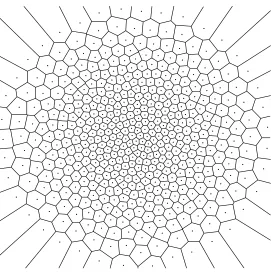
![Figure 3.tessellation, W-quantization (�� Optimal NN = 250) ofW1, supt∈[0,1] Wtdepicted with its Voronoi standard Brownian motion (with B](https://thumb-us.123doks.com/thumbv2/123dok_us/10066049.1992963/39.612.92.483.130.373/figure-tessellation-quantization-optimal-wtdepicted-voronoi-standard-brownian.webp)