Job Displacement and Crime:
Evidence from Danish Microdata
∗Patrick Bennett† Amine Ouazad‡ April 2016
Abstract
This paper matches a comprehensive Danish employer-employee data set with individual crime information (timing of offenses, charges, convictions, and prison terms by crime type) to estimate the impact of job displacement on an individual’s propensity to commit crime. We focus on displaced individuals, i.e. high-tenure workers with strong attachment to their firm, who lose employment during a mass-layoffevent. Pre-displacement data suggests no evidence of endogenous selection of workers for displacement during mass-layoffs: displaced workers’ propen-sity to commit crime exhibits no significantly increasing trend prior to displacement; and the crime rate of workers who will be displaced is not significantly higher than the crime rate of workers who will not be displaced. In contrast, displaced workers’ probability to commit any crime increases by 0.52 percentage points in the year of job separation. The effects are driven by the propensity to commit property crime, which increases by 0.38 percentage points, or about 26% of the population-wide average. The substantial post-displacement earnings losses, coupled with the effects on property crime, are consistent with Becker’s (1968) economic theory of crime. Marital dissolution is more likely post-displacement, and we find small intra-family externalities of adult displacement on younger family members’ crime. The impact of displacement on crime is stronger in municipalities with higher capital and labor income inequalities.
∗We would like to thank Maria Guadalupe, Birthe Larsen, Jay Shambaugh, as well as the audience of the London
School of Economics, the Rockwool Foundation, the INSEAD Symposium 2014, for fruitful comments on preliminary versions of this paper. The authors acknowledge financial and computing support from Copenhagen Business School, INSEAD, and New York University. The usual disclaimers apply.
†Copenhagen Business School. ‡Ecole polytechnique, Paris.
1 Introduction
The causal estimation of the determinants of crime is a central focus of economics. Such determinants are a key input for policymaking, as crime causes significant private and social costs (Anderson 1999),
and affects voters’ perceptions of politicians’ effectiveness (Arnold & Carnes 2012). Additionally,
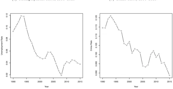
understanding the drivers of crime is a litmus test for behavioral theories, such as Becker’s (1968) theory of crime, which argues that a core motive of criminal behavior is an individual comparison of benefits and opportunity costs. There is, however, disagreement on crime’s specific drivers. While descriptive statistics suggest a broad coincidence of the timing of the peaks in unemployment and the peaks in crime rates (see Figure 1 for Denmark), Levitt (2004) lists the economy as one of the
factors that have too small an effect on crime to explain the 1990s crime rate spike and decline. On
the other hand, a substantial body of literature (Gould, Weinberg & Mustard 2002, Öster & Agell 2007, Fougère, Kramarz & Pouget 2009) finds economically significant impacts of unemployment on crime using credible instrumental variable strategies that predict unemployment rate fluctuations at
the area-level: U.S. states and counties, Swedish municipalities, and French departements.1
Area-wide estimates of the impact of the unemployment rate on aggregate crime are
policy-relevant, as such estimates capture spillover effects as well as direct effects; an important challenge
is to identify what, in such area-wide estimates, is due to the direct impact of individual unemploy-ment on individual crime. Indeed, explaining changes in aggregate crime rates through changes in individual criminal activity is an active area of research (Cook, Machin, Marie & Mastrobuoni 2013). Individual estimates nevertheless require a combination of longitudinal data on unemployment spells, employment spells, and criminal activity with an identification strategy that uses arguably exogenous determinants of job separations.
This paper estimates the impact of job separations on the propensity to commit crime using a unique 1985-2000 employer-employee panel of all prime-aged male individuals in Denmark born
from 1945-1960, matched with crime records (offenses, charges, convictions, and prison terms), with
the timing of unemployment and social assistance spells, and with family identifiers. Given that
1Previous aggregate studies have found significant and modest impacts of unemployment on total (Gould et al.
2002, Öster & Agell 2007) and property (Raphael & Winter-Ebmer 2001, Lin 2008, Fougère et al. 2009) crimes, where a one percentage point increase in the unemployment rate increases total crime by around 5-6% and property crime by around 3-7%. Fougère et al. (2009) finds a one percentage point increase in the youth unemployment rate increases burglaries by 16-35% and auto theft by 22-25% while Falk, Kuhn & Zweimüller (2011) finds a one percentage point increase in the unemployment rate increases right wing extremist crime by 10-20%.
unemployment and social assistance records follow more than 99% of individuals in Denmark, the longitudinal panel provides a comprehensive, almost balanced, panel of individuals since 1985. The data measures recipiency of unemployment benefits at weekly frequency, and crime events at daily frequency. This allows us to determine the specific timing of job separations and criminal activity to single out criminal events happening after the job separation within a given year. Further the
paper records the day of the offense separately from the day of the charges and the day of the
conviction, which is key in eliminating observations for which crime drives job separations rather than separations driving crime.
We focus on job separations for displaced workers: high-tenure workers who experience job
sep-aration during a mass-layoff event, i.e. an event in which a firm loses more than 30 or 40% of its
workers relative to either the firm’s peak employment in 1985-1990, the firm’s average employment in 1985-1990, or relative to a firm-specific trend in 1990-1994 predicted using 1985-1990 employment levels. Using year-to-year declines in firm size of more than 30% relative to firm-specific employment trends allows this paper to consider firm size changes that are arguably sudden and unexpected. As the longitudinal panel follows individuals over time and across municipalities, this paper’s identifi-cation strategy can additionally control for individuals’ non-time-varying unobservables that drive crime and are correlated with displacement, and for municipality-level confounders such as spatial variation in crime-related expenditures or spatial variation in crime-reporting levels.
Displaced workers experience no significant upward trend in their propensity to commit crime prior to displacement; estimated pre-trends display neither statistical nor economic significance. Additionally, displaced workers’ propensity to commit crime prior to displacement, in 1985-1989, is not significantly higher than for individuals with similar tenure who will not be displaced. Such placebo tests therefore do not provide evidence of endogenous separation of high tenure workers
during mass-layoff events.
The paper finds that job displacement leads to significant impacts of displacement on the proba-bility of committing crime. The probaproba-bility of committing crime increases by 0.52 percentage points in the year of displacement, by 0.5 percentage points a year after displacement, and by 0.46 percent-age points four years after displacement. Such displacement events thus raise displaced individuals’ crime rates from below the national average (1.33% for high-tenure workers vs. 1.6% for the national average of males in 1989) to a crime rate above the national average (1.85% post-displacement vs. a
national average of 1.6%). Results are driven by workers with at most a high school education: post-displacement, high-tenure displaced workers with a low level of education typically do not regain employment with similar duration, and experience short-, medium-, and long-run earnings losses of up to 69% of a standard deviation. In line with Becker’s (1968) theory of crime, empirical results
suggest that the paper’s main effects are driven by property crime: the probability to commit
prop-erty crime increases by 0.38 percentage points in the year of displacement, by 0.36 ppt a year after displacement, and by between 0.25 and 0.56 percentage points two to seven years after displacement. The results are robust to a variety of alternative specifications: specifications with a saturated
set of individual, municipal, and year fixed effects; with time-varying controls for changes in marital
status, income, and the number of children; and using alternative mass-layoff definitions. In
partic-ular, a potential concern with using a 30% decline in employment relative to the firm’s 1985-1990 peak or average employment is that firm size may be declining slowly rather than in a sudden and
unexpected way. A corresponding robustness check defines a mass-layoffevent as a 30% reduction in
firm size relative to a firm-specific trend in employment, estimated on 1985-1990 firm size data, and extrapolated to the 1990-2000 decade. While the use of such firm-specific trend halves the number
of measured mass-layoff events, estimates of the impact of displacement on crime are left virtually
unchanged. Results are robust to either a 30% or a 40% threshold for firm size changes as a
defi-nition of mass-layoff events, which mitigates concerns that 30% declines may capture idiosyncratic
firm size changes; and results are robust to considering firms larger than 50 workers.
After estimating the direct impact of job displacement on individual crime, a natural extension is to understand how displacement events interact with the individual’s family. In particular, the paper
estimates whether displacement affects family structure, and whether family structure mitigates the
effects of displacement on crime. The paper’s baseline results are significant regardless of family
structure, i.e. regardless of whether the individual is single, has one or more children, and is in a couple in 1989. However, the impact of displacement on crime is about three times higher for individuals who were single male adults, a finding consistent with the hypothesis that intra-family
income pooling may offer partial consumption insurance post-displacement. Evidence does not
suggest a change in spousal work hours or income in response to the individual’s displacement. The probability of marital dissolution increases post-displacement, with a decline of about 0.9 percentage points in the probability of being married in the year of displacement and of 3.5 percentage points
seven years after displacement. The data suggest some potential but small impact of adult family members’ displacement on son’s crime with a lag, a year after the displacement event.
The importance of municipality-level factors such as income inequality and poverty are also examined. Tax data on wage and capital income enable the construction of income inequality and
poverty concentration measures for each of the 270 municipalities.2 While Denmark as a country
exhibits low income inequality (Atkinson & Søgaard 2013, Piketty 2014), within Denmark the five
most unequal municipalities have a Gini coefficient about twice the Gini in the five least unequal
municipalities. In a cross section, municipalities’ Gini coefficients are not significantly correlated
with either total or property crime rates. Idiosyncratic job displacement causes a post-displacement decline in the individual’s income percentile at the municipal level of about 2.8 percentile points in the year of displacement, and of 3.3 percentile points seven years after displacement. Moreover, displaced workers residing in municipalities in the upper quartile of the Gini distribution are about twice as likely to commit crime post-displacement than workers residing in the lower quartile of the Gini distribution. Importantly, workers in the Copenhagen city area, i.e. those in the municipalities of Copenhagen and Frederiksberg, are not driving the results.
The findings at the individual, family, and municipality levels should be relevant to policymakers and researchers alike. As the data links the employee with his corresponding peers in the family and the municipality, the paper allows an estimation of the impact of job separations beyond its impact on
the employer-employee pair. The paper’s results suggest that firms’ mass-layoffs lead to an increase
in the probability of offenses, charges, convictions, and prison terms, which have corresponding social
costs for victims, as well as policing, prosecution, and incarceration costs. As such, job separations
are unlikely to be efficient (Blanchard & Tirole 2008). Further, higher incarceration rates likely
worsen individuals’ employment prospects: earnings losses for displaced individuals committing a
crime and convicted to prison are substantially higher than earnings losses for similarly displaced
individuals committing a crime but whose conviction does not lead to incarceration.
The paper contributes to at least three literatures. First, seminal papers have estimated the impact of job displacement on earnings (Jacobson, LaLonde & Sullivan 1993), health (Black, De-vereux & Salvanes 2012), mortality (Sullivan & von Wachter 2009), family structure (Charles &
2The paper uses the pre-2007 definition of municipalities, which yields areas of average size 155km2, smaller than
Figure 1: Descriptive Comparison – Unemployment and Crime Rate
Crime Rate: total number of reported crimes over total Danish population. Source: combined register data, supplemented with Statistics Denmark’s STRAF20 statistic. Unemployment rate: male and female as a fraction of labour force as of January 1, from AULAAR. Population on 1. January, from FOLK2.
(a) Unemployment Rate, 1990–2015
● ● ● ●● ● ● ● ● ● ● ●● ●● ● ● ● ● ● ● ● ●● ● ● 1990 1995 2000 2005 2010 2015 0.02 0.04 0.06 0.08 0.10 0.12 Year Unemplo yment Rate (b) Crime Rate, 1990–2015 ● ● ● ● ● ● ● ● ● ● ● ● ● ● ● ● ● ● ● ● ● ● ●● ● ● 1990 1995 2000 2005 2010 2015 0.090 0.095 0.100 0.105 0.110 0.115 0.120 Year Cr ime Rate
Stephens Jr. 2004), children’s school performance (Rege, Telle & Votruba 2011), and regional mo-bility (Huttunen, Moen & Salvanes 2015). To our knowledge, crime is a yet unexplored outcome of job displacement, as records of criminal events, such as data from the FBI’s Uniform Crime Reports (UCR) or the National Incident-Based Reporting System (NIBRS), are typically hard to match with employer-employee data sets. Denmark’s collection of multiple sources of comprehensive reg-istry data, linked together by individuals’ Central Person Register numbers, is a unique opportunity to understand the timing of crime and employment spells. In Denmark unemployment benefits and social assistance recipiency data cover more than 99% of Danes after a job separation, which provides an almost balanced panel data set that bridges the typical data gap between employment spells. The paper combines the job displacement literature and economics of crime as results suggest that earnings losses in the formal sector cause increased property crime. Denmark and other countries
studied in prior literature, in particular the United States, differ in their judicial and labor market
relatively high unemployment benefits (Andersen & Svarer 2007) and lower crime rates (Lavrsen & Pedersen 2013) suggest that the paper’s results are a lower bound of the impact of job displacement on crime. Finally, the paper presents novel results that document costs of incarceration above and beyond the direct costs of incarceration and parole supervision. Indeed, higher incarceration rates may lead to more substantial earnings losses: Individuals who are convicted to prison experience earnings losses of up to 14,000 Danish Kroner (constant 2000 Danish Kroner, 8% of an S.D.) higher than individuals who are convicted to another outcome than prison (suspended sentence, fine, or settlement).
The paper also contributes to the literature on the economics of crime. While prior literature has estimated the impact of changes in the unemployment rate due to changes in the industrial structure of states or counties (Gould et al. 2002, Lin 2008, Fougère et al. 2009), this paper uses a subset of idiosyncratic job separations to estimate the impact of individual displacement on
indi-vidual crime probabilities.3 The Appendix presents a simple job search model4 that formalizes the
difference between the area-wide approach based on unemployment rate fluctuations and the
ap-proach based on individual separations. The former literature uses variations in the unemployment
rate that correspond to simultaneous changes in the arrival rate of offers, the separation rate, and
the distribution of offered wages. The paper’s approach instead focuses on isolating the impact of job
separations during a mass-layoff event on crime. As our treatment effects are estimated relative to
other workers’ crime rates in the same year and the same municipality (includes year, municipality,
and individual fixed effects), the paper isolates the impact of job separations from the impact of
changes in the demand for labor (changes in the economy-wide arrival rate of offers and changes in
the wage distribution).
Third, the paper speaks to the literature on the consequences of income inequalities on an area’s
crime rate. Brush (2007) and Choe (2008) show that, in the cross-section and in first-differenced
panel, income inequality is significantly correlated with crime. Kelly’s (2000) results suggest a significant correlation between inequality and violent crime, but not between income inequality and property crime. Bertrand & Morse (2013) finds that exposure to higher consumption levels by
3In addition to literature examining the impact of unemployment on crime, previous studies have examined the
link between other economic conditions and crime such as wages (Grogger 1998, Machin & Meghir 2004), time spent in unemployment (Bindler 2015), and the impact of graduating during a recession on crime (Bell, Bindler & Machin 2014).
4The mechanism is formalized in a framework as in Stigler (1961) and McCall (1970). The mechanism could be
higher-income households leads to higher individual consumption levels. Such results are consistent with economic theories of interpersonal comparison and envy (Veblen & Mills 1958), which, when confronted with Becker’s (1968) economics of crime, should predict across-municipality variation in
crime rates driven by differences in income distribution. The availability of data on the geographic
location of residence together with income tax data allows us to combine individual trajectories with area-wide data. The paper’s results suggest that, as individuals experience displacement, they are more likely to engage in crime post-displacement if they live alongside higher-income peers. Another implication is that crime prevention policies should be both based on individuals and place-based, as displacement impacts on crime are twice as high in municipalities in the upper quartile of the Gini distribution.
The paper proceeds as follows. Section 2 describes the merged employer-employee-unemployment and crime data set from 1985 to 2000. Section 3.1 presents the identification challenges when cor-relating job separations with crime. Section 3.2 then describes the identification strategy using displaced workers as a subset of idiosyncratic job separations. Section 3.3 introduces the pre- and post-displacement econometric specification, and Section 3.4 shows the paper’s main results.
Sec-tion 4 then analyzes (i) how family structure affects the impact of displacement on crime, (ii) whether
displacement leads to marital dissolution, and (iii) whether fathers’ displacement affects children’s
criminal activity. Section 5 measures local income distribution to identify whether displacement has a greater impact on crime in more unequal municipalities. Finally, Section 6 concludes.
2 Data Set
The Employer-Employee, Unemployment, and Crime Data Sets
An estimation of the impact of job displacement on crime at the individual level requires multiple sources of individual longitudinal panel information: employer-employee data, crime data, data on unemployment and social assistance spells, and demographic data. First, while employer-employee data has detailed information on wages, payroll, firm and worker identifiers, it typically does not capture time periods where an individual is either outside the labor force or looking for a job. Indi-viduals may commit crime during these unemployment spells. Second, estimating the impact of job displacement on crime requires information on the criminal history of each individual throughout the
criminal justice system, from the offense to potential convictions and prison time. Third, estimating the impact of job losses on children’s criminal activity requires matched household members and their age, marital status, and family ties.
Danish Register Data, made available by Statistics Denmark, is a database of every individual formally residing in Denmark from 1980-present, which is collected by government agencies. The employer-employee data set is then constructed through five primary sources: (i) the Integrated
Database for Labor Market Research known in Danish as Den Integrerede Database for
Arbejds-markedsforskning (IDA), which follows a worker in employment spells, (ii) the Central Register of Labour Market Statistics, which follows individuals during weekly unemployment spells, known in
Danish as Det Centrale Register for Arbejdsmarkedsstatistik (CRAM) (iii) the Central Police
Reg-ister, which compiles information from the police and the courts, (iv) the Population Registers, with demographic information and household structure, and (v) the Danish Student Register, which provides information on the highest level of education completed and current student status.
Indi-viduals are linked across these different data sources using anonymized individual Central Person
Register (CPR) numbers, present across all data sources.5
The Integrated Database for Labor Market Research (IDA) compiles data reported annually by employers both at the workplace, firm, and employee levels. The employer-level data contains firm identification numbers, unique workplace identifiers, the number of workplaces in a firm, and the number of employees in each workplace. This is matched to the employee data at the firm level which provides information such as information on part- or full-time employment status, an-nual salary earned in the position, information on secondary employment, as well as the workplace identification number. Annual salary is measured as pre-tax earnings resulting from the employer-employee relationship and is annually collected from employers who are required to report all salaries
paid to all employees to the Danish tax authority SKAT.6 All of the employee and employer data
contained in IDA is observed annually, as in the French (Abowd, Kramarz & Margolis 1999) and Pennsylvania (Sullivan & von Wachter 2009) employer-employee data sets.
Danish registry also addresses a common issue with employer-employee data, i.e. the lack of data in-between employment spells. As identifying precisely when an individuals flows into unemployment
5An individual’s CPR number is a national identification number used when interacting with public services, similar
to a social security number in the US.
is crucial for our empirical design, we supplement the IDA file with data on social assistance and unemployment insurance (UI) benefits received by the individual, from the CRAM registry described above. Importantly, all individuals in the sample constructed for the purposes of estimation are eligible to receive either social assistance or UI benefits. Unemployment statuses are observable at a weekly frequency, allowing us to know the first week an individual is receiving either social assistance or unemployment insurance benefits as well as for how long an individual receives these payments. This paper’s annual data set thus aggregates this weekly data on unemployment, and matches them with the individual’s annual data. This allows us to (i) measure the number of
weeks of unemployment per year, (ii) measure whether individuals commit an offense during an
unemployment spell.
Crime data contained in the Central Police Register is a compilation of police and court records. Individuals who are cited or arrested are then formally charged and assigned a police case number. When such a case number is allocated, it is then matched to the charged individual’s CPR number and to the Danish police station within a district that charged the individual. If multiple people
are charged with committing the same crime, we observe that each of the multiple co-offenders are
matched to the same police case number. The data on criminal charges include the day of the offense
and the day charges were filed.
Charges are assigned a code corresponding to the Danish classification of offenses. We sort
offenses into three broad categories: property crimes, violent crimes, and crimes related to driving
under influence (DUI), but also examine total crimes which comprises these three most frequent crime types as well as less frequent crime categories: sexual, narcotics, firearms, tax, unknown and other crimes, and crimes against special legislation. Crimes “against special legislation” include health-related crimes, environmental crimes, violations of construction and housing laws, crimes related to defense laws. Table 1 panel (iv) shows that about 2.27% of the sample is charged in any given year from 1985-2000. A majority of charges translate into a conviction, as 1.91% of the sample is convicted of any crime. The majority of convictions are driving under influence convictions (0.67% of the sample, which is about 0.67/1.91=35% of convictions), and property crime convictions
(0.65/1.91=34%). A minority of convictions are related to violent crimes or other types of offenses.
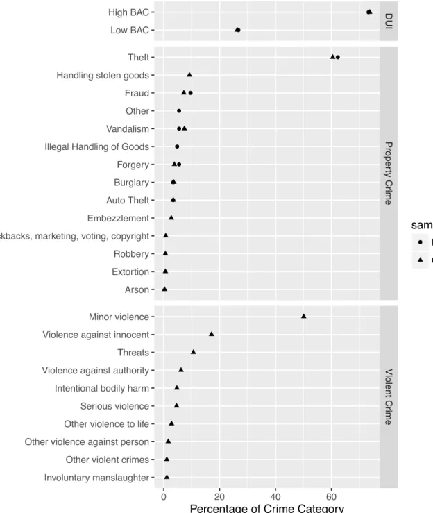
Figure 2 presents a breakdown of crime by subcategory within the broad crime categories. We focus
alcohol contents”, i.e. more than 1.2g of alcohol for every dL of blood. Among property crimes, theft is the largest category, and among violent crimes, minor violence, i.e. violence not resulting in death or injury, is the largest violent crime category. Together with ’violence against an innocent’, these represent more than 2/3 of violent crime, 67.2%.
The police case number follows an individual from charges to courts’ convictions. The Central Police Register includes conviction date and conviction outcome. Such outcome can be either in-carceration, a suspended sentence, a fine, a settlement, no charge/warning, or another less frequent decision such as a youth program or military punishment. While all of these are possible conviction outcomes, the majority of convictions in Denmark result in a suspended sentence, followed by a fine, and incarceration. In what follows, we focus on the first four conviction outcomes, that is
incar-ceration, suspended sentences, fines, and settlements.7 Eventual incarceration dates are recorded
in a similar fashion, with start and end dates, linked to the police case number. Table 2 describes
the timeline from the day of the offense to the day of the charges (upper panel), from the charges
to the conviction (middle panel), and from the conviction to the start of the prison term (bottom
panel). Multiple charges are typically filed for a single offense, hence the large number of charges
(3,729,636) and convictions (1,882,930). In the sample with a least one conviction, charges are filed
the same day as the offense for the median observation. For charges that are not filed the same
day as the offense, the median is at 42 days. About 50.5% of charges translate into a conviction
(second line of the middle panel). Such conviction rate is substantially lower than in other countries such as the United Kingdom, where the conviction rate stood at 82% in 2014 (of Justice of the United Kingdom 2014).
Section 4 below will estimate effects within families and by education. We obtain family and
individual demographic data from the Population Register. Such register is an administrative data
set of all individuals in Denmark, regardless of their labor market status or criminal records. The data include age, gender, municipality of residence, the date the individual’s residence last changed, his immigrant status, marital status, and the mother’s and father’s CPR number. Family members are assigned a family identification number. A household is defined as a set of individuals residing at the same address including any children living at home, with no upper age limit on the children.
7Settlements are described in paragraph 723 of the Danish criminal code, at
To be considered a family, two adults residing together must be registered as a cohabiting couple,
as a married couple, in a registered partnership, or have a common child,8 such that two individuals
sharing a housing unit with no such connection will be considered two families. When either an
individual or family move, their move is self-reported to the Public Registration Office (
Folkeregis-teret). Individuals have significant incentives to report their address changes as these are connected to public services and welfare payments.
The Danish Student Register contains education data such as an individual’s educational qual-ification and educational institution as well as information of any ongoing schooling. For Danes, educational institutions in Denmark are required by law to report this information to the Ministry of Education. We use such administrative education level to categorize a worker’s educational at-tainment into three categories: high school or less education, vocational education, and university education or beyond. The share of non-natives in the early 1990s is relatively small hence measure-ment error in education is unlikely to be a substantial concern (Dustmann, Frattini & Preston 2013).
Merged Longitudinal Data Set
This paper’s merged longitudinal data set links the five above-mentioned sources of longitudinal information to estimate the correlation between job separations and crime. Further sample restric-tions are introduced in section 3.2. As endogenous exit and/or reentry in the sample could be an issue, we focus on individuals who remain in the sample in 1985-2000. In a given year, 0.64% of individuals are not in the data set in the next year, and 0.35% have no observation in the previous year. Results are robust to the inclusion or exclusion of individuals for whom we do not observe
all annual data points.9 We focus on a longitudinal panel of native men in 1985 to 2000. Indeed,
following well-established prior evidence (Freeman 1999), the data set suggests that the majority of
crimes are committed by men, as in Denmark, 86% of all 1985-2000 convictions are given to males.10
The paper estimates the impact of job loss on criminal activity, and focusing on a subset of prime-aged individuals for which labor market participation rates are high. Figure A of the Appendix
8The definition of the statistical concept of a family is provided by the Act on Statistics Denmark §6, Legislative
Decree no. 599 of 22 June 2000.
9Sullivan & von Wachter’s (2009) results indicate that job displacement causes increases in mortality rates. Given
the robustness of our results to the inclusion of individuals without a full 1985-2000 set of observations, it is likely that post-displacement mortality results are relatively unrelated to criminal activity.
10Source: StatistikBanken at Danmarks Statistik (http://www.statistikbanken.dk/); convictions for all types of
suggests that birth cohorts from 1945 to 1960 are birth cohorts for which the employment rate is high and relatively stable. The employment rate increases for cohorts up to the 1943 birth cohort. While 72% of males of the 1926-1944 cohorts are employed in 1990, such employment rate is 87% for the 1945 birth cohort in 1990. On the other end of the age distribution, for younger individuals, focusing on the 1960 and prior cohorts also focuses on individuals with stable attachment to the labor force. While only 78% of males in the 1961-1972 cohorts are employed in 1990, the employment rate is 83% for the 1960 birth cohort.
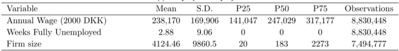
Table 1 presents descriptive statistics for our merged longitudinal data set of Danish males born in 1945-1960 continuously in the panel from 1985 to 2000; the variables are broken down into
each of the five sources. The total number of individual⇥year observations is 8,830,448 or 551,903
observations per year. The median individual earns a wage of 247,029 Danish Kroner (37,310 USD
in 2016),11 and works in a firm with 183 employees. The weekly unemployment data set, collapsed
at the annual level, provides the number of weeks of unemployment. The average number of weeks of unemployment is 2.88, which is about a 5.5% year-round-equivalent unemployment rate. Highest education levels achieved are recorded in the data set for 98.51% of the data set, with 1.49% missing. The median individual contributes 53.76% of his family income, with a median household size of 3 composed of 2 adults and 1 child in the family.
Panel (v) of Table 1 presents data on weeks spent receiving unemployment insurance and social assistance payments for individuals with at least one week of unemployment. The median unem-ployed individual spends 12 weeks on benefits. Although joining an unemployment insurance fund is voluntary, more than 90% of workers aged 30-45 (our 1945-1960 cohorts) were part of a fund in 1990-1995 (Parsons, Tranaes & Lilleør 2015). But Parsons et al. (2015) reports that there are
signif-icant adverse selection effects into unemployment funds, whereby the generosity of social assistance
benefits tends to lower enrollment rates in unemployment insurance funds. Thus, in this paper, we count an individual as unemployed in a given year either if he receive unemployment benefits or if he receives social assistance benefits. Social assistance (first line of panel (v)) is a means-tested social safety net for individuals not enrolled in an unemployment insurance fund. The panel reports the number of weeks on social assistance for individuals with at least one week of social assistance
11Individuals with no wage from employment, excluding all other sources of income enter as zero on this line of the
recipiency. In 1995, less than half a percent (0.45%) of the workforce were looking for work but did
not receive unemployment compensation nor were registered at the unemployment office (Parsons
et al. 2015). Such 0.45% of the workforce are individuals who are not eligible because of high capital income, family assets or spousal earnings, those who voluntarily choose not to claim the benefits even though they are eligible, or those who have been on the benefits so long their eligibility has expired. As the majority of the workforce is covered by either scheme, together with the employer-employee data provides a longitudinal sample of individuals in the Danish workforce.
3 Empirical Strategy
This section documents the endogeneity of individual transitions into unemployment (Section 3.1),
focuses on firms experiencing mass-layoffs and on displaced workers as an identification strategy to
estimate the impact of job separations on crime (Section 3.2), presents this paper’s main econometric specification (Section 3.3), and presents its estimation results (Section 3.4).
3.1 Sample Correlations and Confounding Factors
Table 3 presents correlations between transitions into unemployment and crime using the sample described in Section 2. This table is purely descriptive, and will help in defining the identification challenges when estimating the impact of job loss on criminal activity.
Column (1) of the table presents the OLS regression of a Crime indicator variable on a set of
annual pre- and post-transition into unemployment dummies.12 We focus on the individual’s first
transition into unemployment in the 1985-2000 period. As we observe unemployment status at the weekly level the data set provides the year in which the individual first experienced unemployment. The specification includes all year-level unemployment dummies and thus the average value of the
unemployment dummy coefficients will be equal to the average impact of unemployment on crime.
TheCrime indicator variable is defined as follows. It is set to 1 in yeart= 1985,1986, . . . ,2000
if the individual commits a crime (offense) in yeart that will then lead to a conviction in any year
t0 t. The date of the offense is entered by police staff either at the time a crime is reported to the
12All throughout the paper, and in particular in the displacement regressions of subsequent Section 3.3, we use
linear probability models for the sake of clarity. Linear probability models yield in this paper results that are very similar to the marginal effects of logit regressions, with or without individual fixed effects.
police, or, at the latest, when charges are brought.
Focusing on the timing of the offense rather than the timing of the conviction helps alleviate
concerns of reverse causality, that is an offense which results in job loss. Using the timing of the
conviction could indeed lead to capturing cases where the individual commits an offense, which lead
to both a change in the worker’s employment status and to a conviction. We thus only consider the
timing of offenses.
Focusing on offenses leading to a conviction rather than simply offenses also helps alleviate issues
related to the measurement of a large volume of minor crimes or due to differences in reporting
behavior across police districts. Table 3, columns (1) and (2) use total crimes, including property, violent, and D.U.I. crimes as well as the other crime types discussed in Section 2, as a dependent
variable. Columns (3) and (4) set Crime = 1 when an individual commits and is convicted for
a property crime only. Standard errors are two-way clustered at both the year and the individual levels (Cameron, Gelbach & Miller 2012).
Columns (1) and (3), which do not include an individual fixed effect, suggest that, while crime is
statistically and economically significantly higher post-transition into unemployment, the probability of committing crime is also higher pre-transition into unemployment. Columns (2) and (4) include
an individual fixed effect in the regression. Such an individual fixed effect captures non–time-varying
unobservables that cause both transitions into unemployment and criminal activity. In columns (2)
and (4) as well, significant pre-transition-into-unemployment effects are observed.
Overall, columns (1)–(4) strongly suggest that any identification strategy aiming at identifying thecausal impact of job loss on crime should address the issue of both non–varying and time-varying unobservable confounders.
Table 4 correlates a simple set of observable characteristics with the transition into unemployment indicator variable (column (1)) and the total crime variable (column (2)). Four characteristics (marital status, tenure, firm size, age) are time-varying observables. For the observables of this table, the sign of the correlation with the transition into unemployment is the same as the sign of the correlation with criminal activity. This suggests that the unobservable characteristics are also likely correlated in the same way with displacement and crime; and thus the results of table 3 are likely overestimating the impact of job loss on crime.
3.2 Displaced workers
This paper addresses the issue of the endogeneity of job separations by directing attention on dis-placed workers, in a similar way as in Jacobson et al. (1993) and Sullivan & von Wachter (2009). In this paper, a displaced worker is a high-tenure individual losing employment during a firm’s
mass-layoff event. This section defines both high-tenure individuals and mass-layoff events, leading to a
sample of an arguably idiosyncratic set of job separations.
Mass-Layoff Events
In the period of analysis (1985-2000), prior literature has described evidence of the impact of the Nordic Financial Crisis (Jonung 2008) and of import competition on employment in Den-mark (Ashournia, Munch & Nguyen 2014).
In this paper, we use three different approaches to pinpoint firms experiencing a mass-layoff
event. All three approaches considersudden andunexpected changes in firm13employment relative
to a reference point. What differs across these definitions is the reference point: (i) the peak of
firm employment in the pre-displacement period 1985-1989 as in Jacobson et al. (1993), (ii) the average firm employment in 1985-1989, (iii) a firm-specific trend to predict firm employment levels
in 1990-2000 given the annual employment levels of each firm in 1985-1989. A mass-layoff event
occurs when firm employment is 30% below its reference point, (i)–(iii), depending on the definition. 30% is a threshold that corresponds to the 10th percentile of the distribution of year-to-year change
in log firm size.14 We also consider a higher 40% threshold later in this paper, to avoid capturing
idiosyncratic fluctuations in firm size. The analysis proceeds with private sector firms, for which a
mass-layoff event is more likely to be driven by firm-specific factors than for public-sector firms.
One concern with using peak employment or average employment in 1985-1989 (Definitions using (i) and (ii) as the reference point for employment) is that some firms may be shrinking in size across time and that the 30% change may not be unexpected. Using a firm-specific trend as reference point (definition (iii)) helps alleviate such concern by building a predicted firm size for
firms whose employment is declining. We build the firm-specific trend as follows. Note nj,t the
employment of firmj in yeart= 1985, . . . ,1989, and for eachj= 1,2, . . . , J estimate the regression
13The paper considers firm level downsizing rather than plant-level downsizing as in Jacobson et al. (1993). 14Most log firm size changes are between
±8%: the lower quartile of year-to-year changes in firm size is 6.9%, the median firm experiences no change in employment, and the upper quartile is+8%.
nj,t =↵j + j·t+"j,t. When using (iii) as the reference point, firm j experiences a mass-layoff in
year t = 1990,1991, . . . ,2000 if nj,t is 30% lower than the predicted value ndj,t =↵cj + bj ·t when
bj <0 (declining firm), and is 30% lower thannj,1989 when bj >0.
Table 5 presents the regression of firm size on a set of indicator variables for each year pre- and
post-mass-layoff event. Such regression tests whether firm-size decline trends lead to mass-layoff
events, and whether mass-layoffs are the prelude to larger declines or firm closure. In this table the
reference point is the firm’s peak employment in 1985-1989. If a firm experiences multiple
mass-layoffevents, the first such event is considered but the entire set of observations of the firm is part of
the regression. Column (2) includes year fixed effects, and columns (3) and (4) focus on firms with
between 10 and 1,000 employees inclusive in 1989. Standard errors are clustered two-way at the
firm and year level, and the regressions are performed on 573,860 firm⇥year observations. Overall,
pre-mass-layoffannual indicator variable coefficients suggest that using mass layoffand firm-specific
trends in employment substantially alleviates concerns about pre-trends in firm employment, while
post-mass-layoff annual indicator variable coefficient suggest that firms are, on average, 14 to
62-employee smaller post-mass-layoff. The coefficients for Year +1 to Year +5 also suggest that a
substantial share of the shock is permanent, but that the magnitude of the downward shock does not increase over time.
Displaced Workers
Employees leaving a firm that is experiencing a mass-layoff event may not separate at random.
In particular, individuals losing employment during a mass-layoff event may differ in unobservable
dimensions from individuals staying in employment in that same firm. Gibbons & Katz (1991), Lengermann, Vilhuber et al. (2002) and Abowd, McKinney & Vilhuber (2009) argue that workers
experiencing a mass-layoff event are systematically selected.
The second step of our identification strategy is thus to focus the analysis on individuals with a strong attachment to their firm by imposing a set of sample criteria on the sample from Table 1, and
in Section 3.3 to design a test for pre-separation differences across workers. Four criteria are used
to define strongly-attached individuals: first, individuals need to be continuously employed with the same firm from 1987 to 1989, i.e. they have been employed for at least three consecutive years by the firm in 1989. Individuals can have longer tenure in that particular firm. Second, we focus on
individuals in full-time employment, who are less likely to transition in and out of employment for endogenous reasons. Third, the individual needs to be employed in a firm with 10 or more employees in 1989. This firm-size requirement avoids the problem that percentage changes in firm size are much larger for small than for large firms, for the same corresponding absolute change in employment. The firm size requirement also eliminates self-employment. Individuals with two or more jobs between 1987 and 1989 are not considered as their choice of employment may be driven by the comparison of alternative employment options. Fourth, we consider individuals who were not enrolled in education at any point between 1987 and 1989. Imposing these four criteria on the sample of Table 1 results in a final sample of 102,376 high tenure individuals over the period 1985-2000. As mentioned in Section 2, we consider native males belonging to the 1945-1960 birth cohorts, i.e. who are at least 30 years old in 1990, which is likely to yield a lower bound for the true impact of job separations on crime.
Individuals with a strong attachment to their firm, who have high tenure and are older than 30,
are among the least likely to lose employment during a mass-layoff event. Indeed, the correlation
between tenure in the previous year and unemployment in the subsequent year in Table 3 is
statis-tically and economically significant ( 0.108⇤ ⇤⇤), and the correlation between such lagged tenure
and crime is also statistically and economically significant ( 0.073⇤ ⇤⇤). Similarly, the correlation
between age and both transitions into unemployment and total crime are negative and significant
at 1% ( 0.084⇤ ⇤⇤ and 0.039⇤ ⇤⇤ respectively, last line of Table 4).
The mass-layoffevent will be a decidedly unique event in such high-tenure workers’ history if their
probability of job separation increases substantially at the time of the firm’s mass-layoff event. The
mass-layoffis a firm-wide event that affects all workers regardless of their tenure. To understand the
impact of mass-layoffs on the probability of job separation for high-tenure individuals, we estimate
the probability of job separation in 1989 (rather than 1990) for individuals with at least three years
of tenure in 1988 (rather than 1989) and who will be experiencing a mass-layoff event in 1990. The
probability of job separation in 1989 for such high-tenure individuals who will experience mass-layoff
in 1990 was 3.93% in the year prior to mass-layoff. The probability of job separation for high tenure
individuals in their 1990 mass-layoffevent was 4.72%, as compared to, by definition a 30% or higher
probability for the average worker. As the firm’s employment declines by 30% or more, the rate at which high-tenure individuals with a strong attachment to their firm leave their position increases
by 0.8 percentage points.
Displaced individuals are thus individuals with a strong attachment to their firm who are losing
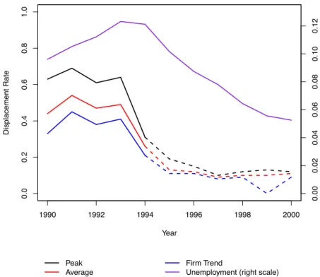
employment during a mass-layoff event. Figure 3 describes the displacement rate in 1990-2000. In
this paper, we estimate the impact of displacement events occurring in the first 5 years of the decade, in 1990-1994 (solid line of Figure 3). The firm trend approach delivers the lowest displacement rate, while the peak employment approach delivers the highest displacement rate. In that sense the firm trend approach is more conservative in that it focuses on firms whose employment changes are sudden relative to the firm-specific trend. Displacement rates range between 0.5% (1990, firm trend definition) and 1.5% (1993, peak definition). The rise in displacement rates in the early 1990s matches the rise in unemployment rates, from 9.61% in 1990 to 12.3% in 1993. The decline in displacement rates from 1993 to 1995 is however steeper than the decline in the unemployment rate in the 1993-1995 period: the unemployment rate declines to 10.2% in 1995 only. This matches the finding that displaced individuals, who have at least three years of tenure prior to displacement, transition to employment with shorter spells and longer durations of unemployment.
A placebo test can estimate whether considering the subset of displaced workers addresses some of the identification concerns that were highlighted in the previous subsection 3.1 and in Tables 3 and 4. Specifically, Table 6 presents a set of regressions of the criminal activity, in 1985 to 1989, of individuals with high tenure in 1985–1989 who will be displaced in 1990–1994. If individuals
who will be displaced differ in their unobservables from individuals who will not be displaced, e.g.
from individuals who will stay in employment during a mass-layoff event, we should observe that
the criminal activity (an offense leading to a conviction) of such future displaced workers is higher
than the criminal activity of individuals who will not be displaced. Column (1) of Table 6 presents such regression for property crime, in OLS and with no additional controls. Column (2) includes
municipality fixed effects and additional controls: indicator variables for education (less than high
school, high school, vocational education, university education or greater), for marital status, control for tenure, firm size, and age. Columns (3) and (4) are the corresponding regressions for violent
crime. Columns (1)–(4) are cross-sectional regressions in 1989, whereF uture Displaced W orker= 1
if the individual will be displaced in any year in 1990-1994. Columns (5)–(8) are regressions pooling all observations in 1985-1989, with a similarly defined right hand side indicator variable. Columns
(5)-(8) add year dummies to control for differences in the crime rates across 1985-1989. Overall the table suggests that future displaced workers are not more likely than non-future displaced workers to
commit a crime in 1985-1989. The coefficients, ranging from 0.00 to 0.08 percentage points, are not
statistically significant at 10%, regardless of the set of controls, year fixed effects, and
municipality-level effects.
The set of crimes leading to a conviction are also similar for the population of displaced workers and for the overall population. Figure 2 presents the distribution of crime types for the overall sample (blue points) and for the sample of displaced workers. Such breakdown is performed for the
overall 1985-2000 data set. D.U.I. offense types are very close for both displaced and overall workers.
For property crime, crime types are ordered by percentage in a similar way among displaced workers and for all workers. Overall results suggest that displaced workers types of property crimes are
similar to the overall population.15
3.3 Econometric Specification
The following baseline specification estimates the impact of displacement on the post-displacement probability of committing crime, controlling for individual-level, municipality-level, and year-level unobservables.
Crimeit =
+7
X
k= 5
k·1(Displaced in year t k) +Individuali
+Y eart+M unicipalitym(i,t)+xit +Constant+"it (1)
where i indexes the N = 102,376 individuals, and t indexes years running from 1985 to 2000.
Crimeit= 1 if the individual icommits a crime in year tand the crime led to a conviction in the
current year or any subsequent yeart0 t. This is defined as in Section 3.1. Focusing on the timing
of the offense, rather than the timing of the conviction or prison term is key to address the problem
of crime affecting separation decisions during a mass-layoff event. Specifically, because we observe
the day of the offense and the week of unemployment, we set Crimeit = 1 so that the day of the
offense always follows the week of displacement.
15The breakdown of violent crime by subcategory for displaced workers is prevented by Statistics Denmark’s
WhileCrimeit = 1implies that an offense leading to conviction has been recorded, charges and convictions typically occur later. Table 2 provides, for individuals convicted, the average, mean, lower and upper quartiles of the duration in days between the day of the arrest or citation and the
day of the conviction. On average the lag is less than a year (172 days) between the offense and
the conviction. Table 2 displays a similar table for displaced, suggesting that the lag for displaced workers is slightly shorter, at 150 days. Combining this timeline of crime with the breakdown of crime by subcategory for displaced and overall (Figure 2) suggests that displaced workers have criminal histories post-displacement that are similar to the overall population.
In specification 1, the coefficient k, for k = 1,2, ...7, is the impact of displacement in previous
year t k on the probability of committing crime in year t. The specification thus allows for
the estimation of short-, medium-, and long-run impacts of displacement on crime, the estimation
includes up to effects 7 years after displacement. The +0 to +6 year effects are identified on all
individuals displaced in our sample, i.e. displaced between 1990 to 1994 inclusive, as our data set
covers year up to 2000 inclusive. The coefficient +7, 7 years after displacement, is identified on
individuals displaced in 1990-1993. With the presence of a constant in the specification, one of the
displacement coefficients is conventionally set to zero; and we choose to set the coefficient 1, a
year prior to displacement, to zero. Thus, as in Table 3, all estimated effects are relative to that
crime rate in the year prior to displacement.
The coefficients for years prior to displacement, 5, . . . , 2 are placebo coefficients; they test
whether high-tenure workers had changes in their propensity to commit crime prior to the
displace-ment event. Statistically significant negative coefficients would be a sign of reverse causality: for
unobservable reasons, future displaced workers would experience an increase in their propensity to commit crime immediately prior to displacement, and such increase in the propensity to commit
crime would be correlated with the probability of losing employment during a mass-layoff event.
Statistically significant positive coefficients, on the other hand, would indicate a dip in crime rates
in the year prior to displacement. Thus checking the absence of economic and statistical significance
of the 5, . . . , 2 is a test of the existence of time-varying unobservable confounders, or, in other
words of the existence of dynamic selection into displacement. Another way to see such identification assumption is to use Wooldridge’s (2010) insight that panel models such as 1 are identified under
that cause crime should not be correlated with future and prior displacement events. The inclusion
of placebo coefficients k can range up to 5 years before displacement, as our data set goes back to
1985 inclusive and follows displacement events from 1990 inclusive.
In subsequent sections we also report cumulative effects: the expected number of years with
at least one criminal event in any year [0; +k] is the sum of the probabilities 0 + 1+ 2 +· · ·+
k. As a criminal event in year t is largely disjoint from a criminal event in year t0 6= t, such
cumulative coefficient is also the probability of committing crime at least once in thekyears following
displacement.
Specification 1 controls for individual-level non–time-varying unobservables through the fixed
effect Individuali. Such unobservables cause crime and may be correlated with the probability
of displacement. For instance, drug consumption is mentioned by Levitt (2004) as a driver of crime; and literature has presented results suggesting a causal impact of psychiatric disorders on job loss (Kessler & Frank 1997). Average drug use over the time period of analysis 1985-2000, could thus be an unobservable confounding factor that causes crime and that is correlated with job losses,
leading to an upward bias on our estimates of displacement. The individual fixed effect controls
for the non–time-varying part of the confounders, and the placebo dummies for the time-varying pre-trends in unobservables. Also, literature has shown that the propensity to commit violent acts can cause job separation (LeBlanc & Kelloway 2002, Grandey, Dickter & Sin 2004), and, separately, that individuals have predispositions to violence (Frisell, Lichtenstein & Långström 2011), potentially
causing both job separation and reported violent crime offenses. Individualifixed effects also capture
individual predispositions to violence.
In our estimation, results suggest that Individuali is negatively correlated with age, education,
and tenure in 1989 and is lower as well for married individuals. As the individual effectIndividualiis
positively correlated with the probability of displacement (+0.010⇤⇤⇤), this suggests thatIndividuali
captures the selection into displacement of crime-prone individuals. The variance of individual effects
is only about 9.6% of the total variance of the crime dependent variable (0.061ppt/0.636ppt),
sug-gesting that dynamic selection into displacement, i.e selection driven by time-varying unobservables
is a substantial concern that will be tested by the placebo coefficients 5, . . . , 2.
Y eart, for t = 1985, . . . ,2000 are a set of year indicator variables that control for national
particular, be correlated with the displacement rate and may confound our estimates of the impact
of displacement on crime. Results suggest that year effects are not statistically significant until
1995, and capture a declining crime rate from 1995 till 2000. Results without year dummies suggest
that not including such national controls tends to bias estimated effects upwards, as the spike in
displacement rates (Figure 3) corresponds to the early part of the sample where crime rates were higher than in the later part of the 1990s.
M unicipalitym(i,t) is a municipality fixed effect, for each of the 270 municipalities,16 where
m(i, t) = 1,2, . . . ,270 is the municipality of individualiin yeart. Municipality fixed effects control
for the existence of municipality-level confounders such as spatial differences in police force numbers
that may be correlated with the occurrence of mass-layoffs; changes in victims’ reporting behavior
at the municipality level; changes in the availability of criminal opportunities that may be
corre-lated with municipality-level displacement rates. The identification of both individual fixed effects
Individuali and municipality fixed effects M unicipalitym is possible given the substantial amount
of individual mobility across municipalities in 1985-2000.
Finally, residuals"it are clustered at the individual level. Results accounting for individual-level
autocorrelation of errors yield similar results and are available from the authors.
Several alternative identification strategies and alternative econometric specifications have been used in the displacement literatures. Dehejia & Wahba (2002) displays an example where propen-sity score matching can be as a good as a randomized experiment and Heckman, Ichimura &
Todd (1997) introduces the Differenced Average Treatment on the Treated strategy. We can
ap-ply such strategy by apap-plying propensity score matching to year-to-year changes in criminal activity
Crimeit 1 Crimeit across displaced and non-displaced individuals in the current year; and by
matching on observables: year of displacement, age, tenure, average income pre-displacement, birth year, education, and marital status. Such matching yields estimates of the impact of displacement on crime ranging between 0.3 percentage points and 0.7 percentage points depending on the match-ing observables, and are consistent with the magnitude, timmatch-ing, and longevity of our main baseline results.
Another approach to the estimation of the impact of displacement on crime is to make use a logit
16Municipalities were consolidated into 98 larger municipalities on January 1, 2007, a phenomenon studied by Amore
& Bennedsen (2013). In this paper we use consistent pre-2007 municipality definitions, which provides a more granular geographic division of the country.
regression model with individual fixed effects instead of a linear probability model with fixed effects. The logit approach is particularly appropriate when one is interested in predicting the probability
of crime, as the estimation approach ensures that probabilities lie in (0,1). However literature has
shown that logit models with individual fixed effects tend to suffer from a lack of consistency of the
estimators due to an incidental parameter problem (Lancaster 2000). The logit approach models
the probability of crime asP(Crimeit= 1) =⇤(P+7k= 5dk·1(Displaced in year t k) +controls).
The estimated marginal impacts ⇤(dk+controls) ⇤(controls) of displacement in yearton crime
k years later are very similar to the estimated impacts k the main specification 1.
3.4 Baseline Results
The results of the estimation of specification 1 are described in Table 7. All regressions of this
table include year, municipal, and individual fixed effects. Column (1) presents the impact of
displacement on total crime, i.e. Crimeit = 1for any crime type. Columns (2)-(3) are for property
crime, Columns (4)-(5) for violent crime, and Column (6) for driving under influence (DUI) offenses.
Columns (1), (2), (4), (6) are the annual impacts k while columns (3) and (5) are cumulative
impacts measuring the impact of displacement on the probability of committing crime in any of
k years post-displacement. All specifications feature the 102,376 individuals over 16 years of the
balanced sample of Danish workers described in Section 3.2. Point estimates are probability increases relative to the year prior to displacement, so that 0.005 corresponds to a 0.5 percentage point increase in the probability of committing crime.
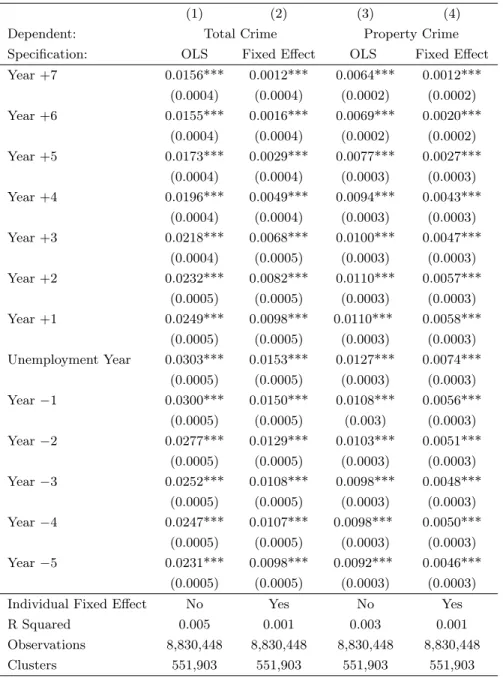
The table suggests statistically significant impacts of job displacement on the probability of com-mitting a crime leading to a conviction. The probability for all crimes increases by 0.52 percentage points in the year post-displacement, and a 0.5 percentage point increase the year following
dis-placement. The effect represents about 0.5/1.91 = 26% of the average probability of a conviction
in the overall population (see Table 1, panel (iv)). Such increase in the probability of committing crime is almost entirely driven by the increase in the probability of committing a property crime. The impact of displacement on crime in the year of displacement is 0.38 percentage points (column (2)), with no discernible impact on the probability of committing a violent crime (Column (4)), and a nonsignificant impact on the probability of a DUI crime (+0.32 percentage points). Figure 2 suggests that for displaced workers these property crimes are mostly theft (62.3%), fraud (9.6%),
forgery (5.5%), and vandalism (5.5%). Together these four subcategories represent 82.9% of all property crimes committed by displaced workers.
Results suggest that the impact of displacement on property crime last beyond the first year: the impact in the year following displacement is +0.36 percentage points, two years after +0.22. Seven years after the displacement event, the probability of committing property crime is still +0.42 percentage points higher than in the year prior to displacement. Figure 4 presents a graphical
depiction of the pre- and post-displacement coefficients of Table7. While the graph suggests a spike
in DUI crimes as well, the curve of total crime and the curve of property crime follow very close trends and levels two years after displacement.
Overall, the average crime rate of future displaced workers in the years prior to displacement is 1.33% for total crime, and 0.13% for property crime; as our sample focuses on individuals with high tenure, these rates are lower than the average for all male workers from the same cohorts, of 1.91% and 0.65% for total crime and property crime respectively. Displacement brings high-tenure workers’ crime rate substantially closer to the average: 7 years after displacement, the crime rates of displaced workers are 1.49% and 0.48% respectively.
Coefficients from Year 5 to Year 2 are not statistically significant at 10% in any of the four
specifications of Table 7. More importantly perhaps is the lack of a discernible trend in point
esti-mates for property crime ( 0.0005in year -5,+0.0002in year -4, 0.0001in year 2) and for violent
crime ( 0.0003 in years 5 to 2). These suggest that individuals who will be displaced are not
experiencing any systematic trends in their propensity to commit crime prior to displacement. Such
lack of evidence of pre-displacement selection effect should alleviate concerns of dynamic selection
and possible reverse causality.
The impact of displacement on property crime, and the lack of impact of displacement on either violent or DUI crimes is consistent at the individual longitudinal-panel level with a substantial body of literature in the economics of crime, both theoretical and empirical with state-level data. Becker’s (1968) theory of crime predicts that individuals compare the cost and benefit of crime, which has led to a vast literature on the impact of unemployment on property crime. Using state-level data, Raphael & Winter-Ebmer (2001) suggests that the decline in property crime can be attributed to
the decline in the unemployment rate in the 1990s.17 Our results, which focus on mass-layoffs,
are also consistent with Mocan & Bali (2010), which finds that the impact of unemployment on crime is asymmetric: Figure 3 indeed suggests that the displacement varies asymmetrically with the unemployment rate: increases in the unemployment rate correspond to much more significant increases in the displacement rate than declines in the unemployment rate. A positive impact of displacement may explain why, then, the response of crime to increases in unemployment is greater than the response of crime to declines in unemployment.
Which individuals are driving our estimates?
Seminal work in the economics of crime considers the young, unskilled, and low-educated males as the main groups of interest (Freeman 1995, Grogger 1998, Gould et al. 2002). The sample of high-tenure displaced workers does include a substantial share of low-education workers: in the sample of displaced workers, 28% of individuals have not finished high school, and about 23.9% are categorized as unskilled workers in the Danish occupational categories. This is to be compared with 27.28% of individuals with less than high school education in the longitudinal sample built in Section 2 and described in Table 1.
Given the importance of educational attainment in determining an individual’s criminal
propen-sity (Lochner & Moretti 2004, Machin, Marie & Vujić 2011, Hjalmarsson, Holmlund & Lindquist
2015), all else equal, we would expect to see larger effects of displacement on crime for displaced
individuals with lower levels of education. Hjalmarsson et al. (2015) uses a credibly exogenous iden-tification strategy relying on changes in compulsory schooling laws to find that one additional year of schooling decreases the likelihood of conviction by 6.7% and incarceration by 15.5%.
While the focus of this paper is to get at an estimate of the causal impact of job displacement on crime rather than estimating the causal impact of education on crime, we can split the sample of displaced individuals to observe which education levels are driving the main results presented in Table 7.
Denmark has two main educational tracks: a general track and a vocational track. In the general track, individuals pursue higher education degrees, while in the vocational track individuals attend schools which are usually combined with apprenticeships. The majority of individuals in the vocational track do not pursue higher education. In the 1945-1960 cohorts that are the focus of this
paper, individuals were required to stay in education until grade 7. In 1975, compulsory education was increased from 7 years to 9 years, the minimum level of education required to pursue additional education in either track. Due to this requirement, most students obtained 9 years of education prior to the reform taking place (Arendt 2005). There are thus three natural categories for splitting the sample by the male individual’s education in 1989: (i) individuals whose highest educational credentials are vocational, (ii) individuals whose highest degree is from the higher education track, and (iii) individuals who have either finished high school but not followed up with the higher-education track, and individuals who have not completed high school. In Denmark, in contrast to the United States, few individuals leave school at the moment of high school completion. Individuals who complete high school typically move on to university education: while 27.23% of individuals in the longitudinal sample have completed less than high school (Table 1), 4.2% have completed high school exactly, 44.33% have completed a vocational degree, and 22.75% have completed a university
degree or more.18
Figure D of the Appendix plots displacement rates by three broad categories of individual edu-cation. The top line (red) is the displacement rate for individuals with vocational eduedu-cation. The middle line (black) is the displacement rate for individuals who have completed high school or less. The bottom line (green) is the displacement rate for individuals who have completed university or more. The displacement rate for workers with vocational education is more than double the dis-placement rate for workers with high school or less than high school (1.3% disdis-placement at the peak vs. 0.6% displacement rate for high school or less).
Table 8 presents the results of the estimation of the main specification 1, where observations are grouped by educational qualification in 1989. Thus such specification estimates the impact of displacement on crime separately for individuals with high school or less, individuals who have completed a vocational education, and individuals with university education or more. Results where the displacement dummies are interacted with the education dummies, rather than results obtained by splitting the sample, are similar and available from the authors.
Table 8 suggests that this paper’s main results are mostly driven by individuals who have com-pleted high school or less. Indeed, for these individuals, the probability of property crime increases by 0.97 percentage points in the year of displacement, more than twice number for the overall sample