https://doi.org/10.5194/wes-3-345-2018
© Author(s) 2018. This work is distributed under the Creative Commons Attribution 4.0 License.
The second curvature correction for the straight segment
approximation of periodic vortex wakes
David H. Wood
Department of Mechanical and Manufacturing Engineering, University of Calgary, Calgary T2N 1N4, AB, Canada
Correspondence:David H. Wood ([email protected])
Received: 7 January 2018 – Discussion started: 17 January 2018 Revised: 13 April 2018 – Accepted: 9 May 2018 – Published: 7 June 2018
Abstract. The periodic, helical vortex wakes of wind turbines, propellers, and helicopters are often approxi-mated using straight vortex segments which cannot reproduce the binormal velocity associated with the local curvature. This leads to the need for the first curvature correction, which is well known and understood. It is less well known that under some circumstances, the binormal velocity determined from straight segments needs a second correction when the periodicity returns the vortex to the proximity of the point at which the velocity is required. This paper analyzes the second correction by modelling the helical far wake of a wind turbine as an infinite row of equispaced vortex rings of constant radius and circulation. The ring spacing is proportional to the helix pitch. The second correction is required at small vortex pitch, which is typical of the operating conditions of large modern turbines. Then the velocity induced by the periodic wake can greatly exceed the local curvature contribution. The second correction is quadratic in the inverse of the number of segments per ring and linear in the inverse spacing. An approximate expression is developed for the second correction and shown to reduce the errors by an order of magnitude.
1 Introduction
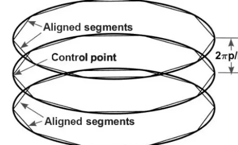
It is common for computational models of the wakes of he-licopters, propellers, and wind turbines to use straight vortex segments whose position is iterated until they follow the lo-cal flow and the vortex is force free. Solving the Biot–Savart integral gives the induced velocity used in the iteration. Fig-ure 1 shows a representation of a vortex trailing from a two-blade rotor with the straight segment approximation. The la-bels and symbols on the figure will be defined below. O’Brien et al. (2017) reviewed a range of computational models for wind turbines and Sarmast et al. (2016) describe a recent ap-plication of a free-wake vortex model using straight vortex segments.
A well-known difficulty of the straight segment approxi-mation is that it does not reproduce the binormal velocity due to the curvature of the vortex line (e.g. Bhagwat and Leish-man, 2014, Govindarajan and LeishLeish-man, 2016, and Kim et al., 2016). This leads to the need for the first curvature cor-rection. To assess the errors of the straight segment
approx-imation and develop a correction, Bhagwat and Leishman (2014) used a vortex ring whose binormal (axial) velocity, U, is given by the well-known Kelvin equation
U= 0
4πlog 8
a
−1
4, (1)
Figure 1.Schematic of two turns of constant radius helical vortices withp=0.1 modelling the far wake of a wind turbine.Nb=2 and the straight segment approximation is shown forNs=10. The flow is down the page. The “control point” is where the induced velocity is required. The contribution from the “aligned segments” on either side of the control point require the largest second curvature correc-tion.
that alter the vortex velocity from its Biot–Savart value: these include flow along the vortex axis, differing distributions of swirl, etc. Nevertheless, the Biot–Savart prescription is use-ful and computationally convenient.
Curvature in the wakes of rotors is often associated with vortex periodicity, the “return” of a vortex to the proximity of the control point, which can cause a significant contribu-tion to the binormal velocity. Wood and Li (2002) and Wood (2004) used helical line vortices to analyze straight segment errors for this second effect of curvature, but their work has apparently not been considered in subsequent vortex mod-elling. Govindarajan and Leishman (2016) claimed that the second curvature correction is unnecessary and difficult to implement. The purpose of this paper is to document the im-portance of the second correction for wind turbine wakes un-der some operating conditions and to develop an effective and simple correction.
The paper is organized as follows. The next section intro-duces the vortex ring model of the wake. In the following section, the induced velocity for the periodic component of the wake over a range of vortex spacings is found in terms of its Biot–Savart integral. Section 4 describes the calculation of the induced velocity for the straight segment approxima-tion, determines the second curvature correcapproxima-tion, and tests its accuracy. The final section contains the conclusions.
2 The vortex ring model for the wake
For a point with the same radius as a single vortex ring and distancezfrom it, the Biot–Savart equation forU in the
di-Figure 2.Vortex ring representation of the helical wake in Fig. 1 and the corresponding vortex segment approximation.
rection of the wind – the binormal direction – is
U= 0
4π
2π
Z
0
1−cosθ
(2−2 cosθ+z2)3/2dθ, (2)
whereθis the vortex angle in cylindrical polar co-ordinates. Ifz=0, the integral clearly has a logarithmic singularity as θ→0. The velocity,U1c, requiring the first curvature
correc-tion is
U1c=U(z=0), (3)
arising from the only ring containing the control point. The integral in Eq. (2) and similar equations will be termed the “influence coefficient”I, which has the same relative error characteristics asU.
The test case used here to investigate the second correction models the far wake of a wind turbine as an infinite row of equispaced vortex rings of constant spacing,s, radius, and 0, extending to infinity on either side of the control point atz=0. A row of rings is easier to analyze than the helical vortices used by Wood and Li (2002) and Wood (2004) but displays the same need at small separation for the second correction. In addition, the discrete nature of the vortex rings helps to localize the correction that is developed in Sect. 4.
The ring vortex wake is consistent with the “Joukowsky” model of the wake, used by Sarmast et al. (2016); either the bound vorticity of the blades is constant along their span or all the shed vorticity has rolled up into tip and hub vortices before reaching the far wake. This is clearly a simplification of wind turbine wakes in general, but the linearity of the Biot–Savart law allows more complex wakes to be consid-ered as an assembly of elements such as rings. The velocity associated with the second correction,U2c, is induced by the
vortices that do not contain the control point:
U2c=
0 4πI2c=
0 4π
2π
Z
0
2
∞
X
j=1
1−cosθ
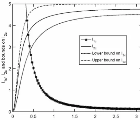
Figure 3.The integrands for the two influence coefficients for a control point on the vortex ring andθ0=0. The stars show the inte-grand forI1cfrom Eq. (2) withz=0. The solid line showsI2c. The dashed and dotted lines are the bounds onI2c, Eq. (5) withs=0.2. The sums were evaluated using Eq. (4) for 50 000 rings.
Equation (4) is not singular asθ→0, which is, possibly, the reason why the need for the second correction has not been appreciated.scan be identified with the pitchpof a helical vortex wake and the number of blades,Nb, according tos=
2πp/Nb. The relationship betweenp ands can be seen by
comparing Figs. 1 and 2.
Testing corrections for the straight segment approximation requires an accurate evaluation of the series in Eq. (4) and then an integration inθ. This order is preferred because the integration inθ of the summand results in incomplete ellip-tic integrals, which are likely to be very difficult to sum. The innocuous looking series in Eq. (4), however, does not ap-pear to have a closed form sum. The standard technique for summing infinite series of algebraic functions is via Laplace transforms (e.g. Wheelon, 1954). This would be successful if the exponent in the integrand was 1 instead of 3/2, but for Eq. (4), the method gave a principal value integral that could not be solved in closed form. By the Cauchy integral test for series
1 s−
1
√
2−2 cosθ+s2≤I2c(θ)≤
1 s−
1
√
2−2 cosθ+s2
+ 2(1−cosθ)
(2−2 cosθ+s2)3/2, (5)
where
I2c=
2π
Z
0
I2c(θ)dθ and
I2c(θ)= ∞
X
j=1
1−cosθ
(2−2 cosθ+(j s)2)3/2. (6)
It is easy to show that the average velocity in the direction of the wind at any radiusr <1 within the Joukowsky wake is 1−0/s(e.g. Wood, 2011), and it is reasonable to assume that the total velocity of the free-wake vortex rings is close to 1−0/(2s) or the induced velocity,U≈0/(2s). Further, the bounds in Eq. (5), which both contain 1/s, causeUto ap-proach the average of the wake and external velocities, pro-vided the curvature singularity does not contribute signifi-cantly toU. There is, unfortunately, only limited experimen-tal information ona andU for wind turbine wakes to guide the assessment of the relative importance of the first and sec-ond velocity fields and their corrections. Figure 3 shows the terms in Eq. (5) fors=0.2. This typical value was obtained using the following steps. For modern turbines,Nb=3, and
λ≈7 for most of the operating range. For optimal (Betz-Joukowsky) performance,U=1/3,p≈2/(3λ), whereλis the tip speed ratio, andNb0λ/π=8/9 (Wood, 2011). Thus
0=0.133 ands≈0.2. The sum in Eq. (4) is always zero whenθ=0, but, ass decreases, the bounds in Eq. (5) (and hence the sum) tend to 2π/s over an increasing range of θ. Integrating over[0,2π]then leads toU≈U2c≈0/(2s),
showing the potential importance ofU2c. The integrand of
I1cfor a smallθis also shown. Its integral andU1cdepend on
the cut-off,a; to matchU=2/3 for the conditions in Fig. 3, Eq. (1) requiresa∼10−23, which does not seem a reason-able value. Thus it is likely thatU≈U2cat the smallpands
typical of the operating conditions of modern wind turbines. The very limited experimental information on the velocity of the vortices in wind turbine wakes are in general agree-ment with this arguagree-ment. Xiao et al. (2011) measured the wake of a two-bladed turbine in a wind tunnel atλ=4.91 using particle image velocimetry. They determined the vor-tex velocity in the near wake as 10.8 m s−1 when the wind speed was 12 m s−1. ThusU=(12−10.8)/12=0.1, which is lower than the value of 1/3 that follows from assuming optimal power output. AssumingU=U2cand using the
gen-eral equationp=(1−U)/λgivess=0.576 or 360 mm for the rotor of radius 625 mm, which agrees very well with the value read from their Fig. 10. This again implies that U2cU1c. Since most rotor wakes are helices of some form,
it is important to note that the equivalent inverse pitch term dominates U for a helical vortex of sufficiently small p (Kuibin and Okulov, 1998). There is a further reason to ex-pectU≈U2cU1cfor many turbine wakes: U1c, but not
U2c, is associated with the impulse necessary to form a
vor-tex ring. If that impulse andU1care significant it is unlikely
array of vortex rings
A closed form sum forU2cin Eq. (4) could not be obtained
so the influence coefficients for a range of s values were determined as follows. The Hermite–Hadamard inequality for monotonically decreasing functions that tend to zero at large argument can be used simply to give a tighter bound on I2c(θ). It is
I2c(θ)=
1 s−
1
√
2−2 cosθ+s2+
1−cosθ
(2−2 cosθ+s2)3/2+δ(θ),
(7)
where the difference,δ(θ), is always positive but must be de-termined numerically. The integral of the other terms on the right side of Eq. (7) can be found exactly:
2π Z 0 1 s− 1 √
2−2 cosθ+s2+
1−cosθ (2−2 cosθ+s2)3/2
dθ
=2π
s −
2sE(−4/s2) s2+4 −
2K(−4/s2)
s , (8)
where E(.) and K(.) are the complete elliptic integrals in standard notation. The difference,δ, the integral ofδ(θ) over
[0,2π], was evaluated using 2000 increments ofθand num-ber of rings, Nr=50 000. This value was chosen using the
result obtained from Mathematica, that
2π Z 0 2 ∞ X
j=Nr
1−cosθ
(2−2 cosθ+(j s)2)3/2dθ
→R(Nr)=
4π ζ(3)−HN(3)
r
s3 (9)
for large Nr, where ζ(.) is the zeta function, and H is the
harmonic number in standard notation. In later use of this re-sult,R(j) will be called the “remainder”. Using 2π/sas an estimate for the integral in Eq. (4), and using Mathematica to evaluateH3(Nr), gave the relative error in truncating the sum
atNr=50 000 as 2/s2×10−10=2×10−8for the smallest
value ofsconsidered here,s=0.1. To the number of decimal places used in Table 1, truncation does not alter the integral of the terms in Eq. (7) over[0,2π]. For every calculation up to Sect. 5,Nr=50 000. Theθ−integral of the sum in Eq. (7)
was found using the MATLAB quadrature routine “integral” with an absolute tolerance of 10−8. All integrands are sym-metric aboutθ=πand so were obtained over[0, π]. Table 1 also shows the approximateλfor a Betz–Joukowsky optimal rotor.δis small: combining Eqs. (6) and (7) leads to
0≤δ≤ 2K(−4/s
2)
s −
2sE(−4/s2)
s2+4 , (10)
which is satisfied by allδvalues in Table 1.δis less than 4 % ofIcfor the worst case ofs=0.8; Eq. (8) is an increasingly
good approximation to the sum and the influence coefficient approaches 2π/sassdecreases andλincreases. The values of I2c in Table 1 will be compared to the values from the
straight segment approximation.
4 Straight segment approximation of vortex rings and its accuracy
Each of the rings not containing the control point was ap-proximated by an even number, Ns, of straight segments.
The ith segment of each ring started at θ=2π i/Ns+θ0
when measured from the control point and finished at 2π(i+
1)/Ns+θ0.θ0is the angular displacement between the
con-trol point and the start of the first (i=0) segment. A straight-forward application of Eq. (10.115) of Katz and Plotkin (2001) givesI2c(i, j), the contribution of theith segment on
the twojth vortex rings toU2c, as
U2c(i, j)=
0 4π
Nr X
j=1
Ns X
i=1
I2c(i, j),where
I2c(i, j)=
AiBi,j
Ci,j
, (11)
and
Ai=8 sin π i
Ns +θ0
2
sin
π(i+1)
Ns
+θ0
2
, (12)
Bi,j=sin π Ns
1
bi+1,j
+ 1
bi,j
+sin
(2i+1)π
Ns
+θ0
1
bi+1,j
− 1
bi,j
, (13)
Ci,j=cos 2π Ns
+b2i,j+b2i+1,j
+cos
2π(2i+1)
Ns
+2θ0
−2, (14)
and
bi,j = s
2−2 cos 2π i
Ns +θ0
+(j s)2. (15)
For the first calculations, the junction of the first andNsth
segment was aligned with the control point soθ0=0. The
in-fluence coefficients calculated from Eqs. (11)–(14) are com-pared to the results from Table 1 in Fig. 4 in terms of the rel-ative error using the integral over[0, π]as the denominator since the integrand must be symmetric aboutθ=π. The er-ror is defined as the exact integral minus the straight segment approximation so the latter is always an underestimate. Two separate ranges ofθare considered: for 0≤ |θ| ≤π/2 the er-ror is 1 to 2 orders of magnitude higher than forπ/2≤ |θ| ≤
Table 1.Values of the influence coefficient for varyingsvalues withθ0=0.
s Approx.λ Equation (8) δ I2c 2π/s
0.10 14 57.448345 0.163716 57.612061 62.831853
0.20 7 26.722916 0.166712 26.889628 31.415927
0.40 3.5 11.703237 0.172962 11.876199 15.707963
0.80 1.75 4.546484 0.174676 4.721160 7.853982
1/N
s
10-2 10-1
Relative error
10-6 10-5 10-4 10-3 10-2 10-1
0≤|θ|≤π/2
π/2≤|θ|≤π
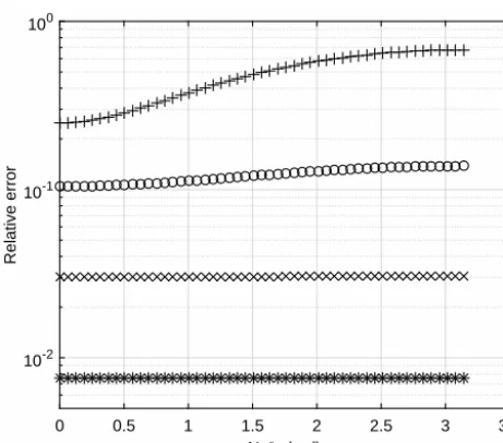
Figure 4.Relative error of the straight segment approximation for the conditions in Table 1 (θ0=0).+:s=0.1;◦:s=0.2;×:s= 0.4;3:s=0.8. The top group of symbols show the errors for the first half of the rings that contain the aligned segments, 0≤ |θ| ≤ π/2, and the bottom group coversπ/2≤ |θ| ≤π.Ns=20,40,80, and 160.
toU2cas the Biot–Savart velocity must lie in the plane
con-taining the segment and the control point. Otherwise, both errors scale as 1/Ns2, as was found in the helix simulations of Wood (2004). As sdecreases, however, the aligned seg-ment error increases proportionally to 1/s, but the error for the remaining range ofθdecreases at constantNs.
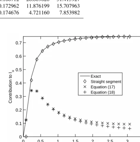
Figure 5 shows the angular contribution to the influence coefficients for s=0.2 and Ns=40. The value of θ used
for plotting is the midpoint of each segment. The solid line shows the exact integral from θi toθi+1. As was found by
Wood and Li (2002) and Wood (2004), the errors are local-ized near θ=0. A correction for the error for the aligned segments can be developed from the small-θ expansion of the series in Eq. (4):
I2c(θ)=2 ∞
X
j=1
I2c(θ, j)= ∞
X
j=1
2−2 cosθ
(2−2 cosθ+(j s)2)3/2
→ζ(3)θ 2
s3 asθ/s→0 (16)
θ (rad)
0 0.5 1 1.5 2 2.5 3 3.5
Contribution to I
u
0 0.1 0.2 0.3 0.4 0.5 0.6 0.7
Exact Straight segment Equation (17) Equation (18)
Figure 5.Angular contribution of straight segments to the influ-ence coefficient forz=0.2,Ns=40, andθ0=0. The value ofθ is the midpoint of the segment. The solid line shows the numerical solution of the exact integral.3shows the straight segment con-tribution,×the contribution from Eq. (17), and+the contribution from Eq. (18).
andζ(3)=1.2026. Equation (16) has two important implica-tions. First, the best possible error for periodic straight seg-ments scales as (Nss)−3but it is likely that an unrealistically
high value ofNswould be required to achieve this. Second,
1/ζ(3) or over 80 % of the correction toU2cis due to the two
rings (j =1) on either side of the control point. This is the justification for pointing out the aligned segments in Figs. 1 and 2. A general form of the correction, therefore, can be based on the returned vortex on either side of the control point. Since the distance from the control point to the vor-tex segments must be calculated in a free-wake simulation, it should not be difficult to determine the proximity in terms ofθ/zand apply a correction. A more general correction is 1(θs), whereθs=2π/Nsis obtained by integrating inθonly
forj =1 and then usingζ(3) to correct approximately for the remaining rings. The result is
1(θs)≈2ζ(3)
F θs/2,−4/s
2
s −
sE θs/2,−4/s2
s2+4
− 2 sinθs
s2+4 p
2−2 cosθs+s2
N
sθ0 (rad)
0 0.5 1 1.5 2 2.5 3 3.5
Relative error
10-2 10-1 100
Figure 6.Variation in relative error withθ0fors=0.1.Ns=20, +;Ns=40,◦;Ns=80,×;Ns=160,?.
where E(.) and F(.) are the incomplete elliptic integrals. Equation (17) is shown in Fig. 3 to give a better estimate for the aligned segments. An alternative, simpler correction than Eq. (17) can be found by using 2−2 cosθ∼θ2for small θvalues to give
1(θs)≈2ζ(3) "
log θ
s+
p θ2
s +s2
s
− θs
p θ2
s +s2
#
, (18)
which gives almost the same correction for the aligned seg-ments; Fig. 5. These results for the application of Eqs. (17) and (18) to the aligned segments are similar at the other val-ues ofsas well, but are not shown in the interests of brevity. It is noted that the correction developed here is simple in the sense that the vortex curvature is known a priori. As pointed out by Govindarajan and Leishman (2016), however, and shown by the analysis of Kim et al. (2016), the modelling of three-dimensional wakes of varying geometry can be con-siderably more complex.
One of these complexities is that the control point may not align with the junction of segments on (in this case) adjacent rings. The effect of this can be investigated by using non-zero θ0 in Eqs. (12)–(15). The results are shown in Fig. 6
for 20≤Ns≤160 and 0≤θ0≤π/Ns ands=0.1. As was
found for other values ofs, there is remarkably little variation in the error withθ0except for the lowestNs, suggesting that
the correction derived above for the aligned case (θ0=0) is
also applicable to other values. This is not an immediately obvious result from Eqs. (12)–(15). Forθ0=π/Ns andθ=
2π/Ns:
I2c(θ,1)=
8sin2(θ/2) sinθ
3−4 cosθ+cos 2θ+2s2√
2−2 cosθ+s2
θ (rad)
0 0.5 1 1.5 2 2.5 3 3.5
Contribution to I
u
0.1 0.15 0.2 0.25 0.3 0.35 0.4
Figure 7.Variation in the straight segment approximation toI2c(θ) forθ0=0 andNr=5,×; 10,◦; 20,;+, 50;×, 50 000.Ns=40,
s=0.2.
→
θ s
3
as θ/s→0, (19)
which suggests a difference from the case whenθ0=0.
5 Using a finite array of rings to determine the influence coefficient
The second curvature error was shown in the last section to be caused largely by aligned segments on the rings either side of the control point. For increasingθ,I2c(θ) becomes
dom-inated by rings at a larger distance from the control point. This is shown in Fig. 7, which implies thatNreither must be
large to ensure an accurate determination ofI2cor a suitable
remainder term be used. This allows an approximate deter-mination of the influence coefficient for the case in which θ0=0 according to
I2c≈21(θs)+
Nr X
j=1
Ns X
i=1
I2c(i, j)+R(Nr), (20)
where one possibility for the remainderR(Nr) is given by
Eq. (9).
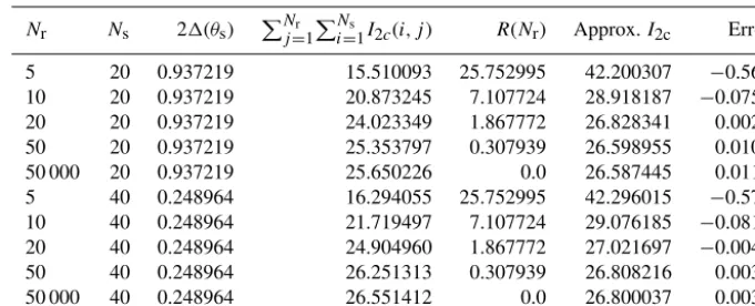
The terms in Eq. (20) are listed in Table 2 fors=0.2. A significant number of vortex rings,Nr, or equivalently a
large stream-wise distance is needed to make the remainder, R(Nr), accurate. Typically,Nr≥20 for thiss, and thenR(Nr)
is comparable to1(θs). ForNs=20, for example, after
Table 2.Terms in Eq. (20) fors=0.2 andθ0=0. Exact value ofI2c=26.889628. The error is the relative error.
Nr Ns 21(θs) PNj=r1PNi=s1I2c(i, j) R(Nr) Approx.I2c Error
5 20 0.937219 15.510093 25.752995 42.200307 −0.569
10 20 0.937219 20.873245 7.107724 28.918187 −0.0754
20 20 0.937219 24.023349 1.867772 26.828341 0.0023
50 20 0.937219 25.353797 0.307939 26.598955 0.0108
50 000 20 0.937219 25.650226 0.0 26.587445 0.0112
5 40 0.248964 16.294055 25.752995 42.296015 −0.573
10 40 0.248964 21.719497 7.107724 29.076185 −0.0813
20 40 0.248964 24.904960 1.867772 27.021697 −0.0049
50 40 0.248964 26.251313 0.307939 26.808216 0.0030
50 000 40 0.248964 26.551412 0.0 26.800037 0.0033
6 Conclusions
The widely used straight segment approximation for approx-imating the curved and periodic vortex wakes of wind tur-bines, propellers, and helicopters can have two errors asso-ciated with the wake curvature. The first is the well-known error in reproducing the locally induced binormal velocity. This is usually accommodated by a cut-off in the Biot–Savart determination of the vortex velocity using Eqs. (2) and (3) at a distance comparable with the radius of the vortex core. The second, less well-known error is the subject of this paper. It arises from the alignment of the segments of the periodic vortex returning to the proximity of the point at which the velocity is being determined.
By modelling the far wake of a wind turbine as an infi-nite row of equispaced vortex rings, two important results were obtained. First, it was shown that the velocity associ-ated with the second error dominates at the small spacings typical of modern wind turbine operation. The available ex-perimental evidence on wake structure is consistent with this finding. Then it is shown that the second error is quadratic in the number of segments per revolution and inversely propor-tional to the spacing of the rings, which is proporpropor-tional to the pitch of a more realistic, but more difficult, helical wake. The model to investigate the second correction is artificial in that a single, infinite row of vortex rings of constant spacing, ra-dius, and circulation is not applicable to the near wake. Nev-ertheless the model demonstrated the general importance of the rings adjacent to the control point at which the velocity is being calculated. These adjacent rings contribute over 80 % of the correction that is needed because the straight segment approximation does not correctly determine the contribution to the induced velocity from the closest parts of the adjacent rings, called the aligned segments.
It was also shown that the best behaviour possible for the second error is cubic in the product of the number of segments per revolution and the vortex spacing. It is likely, however, that larger numbers of vortex segments would be needed to achieve this error than are used in practice. This
result was generalized to develop a second correction that improves the computed induced velocity by nearly 1 order of magnitude.
Code availability. The MATLAB codes used in this study are available from the author.
Competing interests. The author declares that he has no conflict of interest.
Acknowledgements. This work is part of a research project on wind turbine aerodynamics funded by the NSERC Discovery Grants Program.
Edited by: Alessandro Bianchini
Reviewed by: Joseph Saverin and Wang Xiaodong
References
Bhagwat, M. J. and Leishman, J. G.: Self-Induced Velocity of a Vortex Ring Using Straight-Line Segmentation, AIAA Journal, 59, 1–7, 2014.
Govindarajan, B. M. and Leishman, J. G.: Curvature Corrections to Improve the Accuracy of Free-Vortex Methods, J. Aircraft, 53, 378–386, 2016.
Katz, J. and Plotkin, A.: Low-Speed Aerodynamics, 2nd edition, C.U.P., Cambridge, 2001.
Kim, C. J., Park, S. H., Sung, S. K., and Jung, S. N.: Dynamic mod-eling and analysis of vortex filament motion using a novel curve-fitting method, Chinese J. Aeronaut., 29, 53–65, 2016.
Kuibin, P. A. and Okulov, V. L.: Self-induced motion and asymp-totic expansion of the velocity field in the vicinity of a helical vortex filament, Phys. Fluids, 10, 607–614, 1998.
O’Brien, J. M., Young, T. M. O’Mahoney, D. C., and Griffin, P. C.: Horizontal axis wind turbine research: A review of commercial CFD, FE codes and experimental practices, Prog. Aerosp. Sci., 97, 1–24, 2017.
Sarmast, S., Segalini, A., Mikkelsen, R. F., and Ivanell, S.: Com-parison of the near-wake between actuator-line simulations and a simplified vortex model of a horizontal-axis wind turbine, Wind Energy, 19, 471–481, 2016.
Wheelon, A. D.: On the Summation of Infinite Series in Closed Form, J. Appl. Phys., 113, 113–118, 1954.
Wood, D. H.: Method to Improve the Accuracy of Straight-Segment Representation of Helical Vortices, AIAA Journal, 41, 256–262, 2004.
Wood, D. H.: Small Wind Turbines: Analysis, Design, and Appli-cation, Springer, London, 2011.
Wood, D. H. and Li, D.: Assessment of the accuracy of representing a helical vortex by straight segments, AIAA Journal, 40, 647– 651, 2002.