A Comparative Study between a Pseudo-Forward Equation (PFE) and Intelligence Methods for the Characterization of the North Sea Reservoir

(1)

IJMGE

Int. J. Min. & Geo-Eng.

Vol.48, No.2, December 2014, pp.173-190.

173

A Comparative Study between a Pseudo-Forward Equation (PFE) and

Intelligence Methods for the Characterization of the North Sea

Reservoir

Saeed Mojeddifar

1*

, Gholamreza Kamali

1

, Hojjatolah Ranjbar

1

, Babak Salehipour Bavarsad

2

1

Department of Mining Engineering, Shahid Bahonar University of Kerman, Kerman, Iran

2

Geopardazesh Petroleum Exploration Services, Ahvaz, Iran

Received 8 Oct 2014; Received in revised form 22 Nov 2014; Accepted 20 Dec 2014

*Corresponding author:[email protected]

ABSTRACT

This paper presents a comparative study between three versions of adaptive neuro-fuzzy inference system (ANFIS) algorithms and a pseudo-forward equation (PFE) to characterize the North Sea reservoir (F3 block) based on seismic data. According to the statistical studies, four attributes (energy, envelope, spectral decomposition and similarity) are known to be useful as fundamental attributes in porosity estimation. Different ANFIS models were constructed using three clustering methods of grid partitioning (GP), subtractive clustering method (SCM) and fuzzy c-means clustering (FCM). An experimental equation, called PFE and based on similarity attributes, was also proposed to estimate porosity values of the reservoir. When the validation set derived from training wells was used, the R-square coefficient between two variables (actual and predicted values) was obtained as 0.7935 and 0.7404 for the ANFIS algorithm and the PFE model, respectively. But when the testing set derived from testing wells was used, the same coefficients decreased to 0.252 and 0.5133 for the ANFIS algorithm and the PFE model, respectively. According to these results, and the geological characteristics observed in the F3 block, it seems that the ANFIS algorithms cannot estimate the porosity acceptably. By contrast, in the outputs of PFE, the ability to detect geological structures such as faults (gas chimney), folds (salt dome), and bright spots, alongside the porosity estimation of sandstone reservoirs, could help in determining the drilling target locations. Finally, this work proposes that the developed PFE could be a good technique for characterizing the reservoir of the F3 block.

Keywords: ANFIS, clustering algorithms, experimental equation, porosity, seismic attributes.

1. Introduction

The spatial distribution of petro-physical parameters between wells in a hydrocarbon reservoir is an important issue in the petroleum industry. Hence, laboratory

(2)

174 Several studies have shown that the inversion of seismic data into acoustic impedance (AI) is widely used in hydrocarbon exploration to estimate petro-physical properties. The acoustic impedance is commonly applied for porosity estimation, mostly based on an empirical relationship between acoustic impedance and porosity. However, the relationship differs from area to area because the compaction model varies both laterally and vertically. Thus, in many cases, porosity could not be estimated directly from the acoustic impedance using a single transform function in a large area [2].

For this reason, Schults et al. [3] proposed the idea of using multiple seismic attributes to estimate log properties aside from well control. Therefore, various data integration techniques such as kriging or neural networks have been used to directly derive the petro-physical properties from seismic attributes. For example, artificial neural networks (ANN) have been applied to predict core properties from well logs [4], and seismic properties have been employed to predict lithology [5-8], sonic logs and shale content [9], shale stringers in a heavy oil reservoir [10], spontaneous potential [11, 12], permeability [4, 13] and porosity [5, 7, 8, 14-18].

Recently, Adekanle and Enikanselu attempted to improve spatial prediction of petro-physical properties through integration of petro-physical measurements and 3D seismic observations using multiple regression analysis [19]. Lei et al. proposed a dynamic radial basis function (D-RBF) network method to predict the reservoir’s properties from seismic attributes [20]. Eftekharifar et al. developed a method for 3D modelling and interpretation of log properties from complex seismic attributes using principal component analysis and local linear modelling [21]. Hosseini et al. used three types of neural network for inversion of seismic attributes and prediction of reservoir porosity [22]. Basu and Verma attempted to generate effective porosity volume using multi-attribute transform and probabilistic neural network [23]. Valenti compared methods of neural network and multi-linear regression analysis for predicting well-log porosity from seismic data [24]. Joonaki et al. presented an

intelligent approach for the oil reservoir characterization using seismic elastic properties and a physical rock model [25].

In addition to the applied techniques in the aforementioned researches, modern artificial intelligent methods such as neuro-fuzzy systems could be used for the prediction of petro-physical properties. These methods provide fast, reliable and low-cost solutions. Another advantage of these methods is that they can handle dynamic, non-linear and noisy data, especially when the underlying physical relations are very complex and not fully understood. Since artificial intelligence methods have not presented a specific mathematical equation to describe the relationship between attributes and petro-physical properties, this paper implements a non-linear mathematical equation to describe the relationship between a seismic attribute (similarity) and the porosity value, and compares the results with three versions of ANFIS algorithms, which are developed based on different clustering algorithms. This model, which transforms similarity attributes of a sandstone reservoir to porosity values, is called the pseudo-forward equation (PFE) in this paper. The structure of PFE is implemented based on the data set of the gas reservoir of F3 block in the North Sea. This reservoir consists of sand and shale layers. Shale units are sandwiched between the sand layers. Therefore, the role of PFE in both rock types will be investigated. The initial parameters of PFE are unknown and should be derived from the data. This study will use algebra technique to solve the non-linear model, and finally the quality of the implemented model will be compared with the results of ANFIS algorithms.

2. Geological setting

(3)

175 basin was defined by a period of rapid deposition and shallowing of the basin [27]. The most important geological occurrence in that period was the expansion of deltaic systems [26]. The delta systems in the North Sea region can be classified into two groups according to sources of the sediments. Until the

early Pliocene, the main transport factor was the Baltic river system that deposited coarse fluvial sediments. Afterwards, German rivers became the main agent in the North Sea [28]. The Cenozoic sequence could be subdivided into two main packets separated by the mid-Miocene unconformity (MMU) (Fig. 1).

Fig. 1. S ketch of the Neogene fluvio-deltaic system in the southern North S ea (after [29])

The region between the Lower Tertiary and the mid-Miocene unconformities are known as the Lower Cenozoic sequence. The area from the mid-Miocene unconformity up to the sea bottom forms the Upper Cenozoic sequence. The reflections from the layers between the unconformity and the Plio-Pleistocene boundary in the Upper Cenozoic sequence are most interesting for this work. This region is a deltaic sequence subdivided into three sub-sequences (Units 1, 2 and 3). Unit 1 belongs to the first phase of the delta’s evolution above the unconformity. Field evaluations show that their height varies between 4 and 10 ms two-way travel time. Unit 2 belongs to the second phase of delta evolution and consists of

sigmoid progradational reflection

configurations. This unit shows a prograding clinoform pattern formed by superimposed sigmoid reflections. Unit 3 belongs to the final phase of delta evolution. The reflection configurations of the unit are characterized by divergence [30]. The deltaic package consists of sand and shale, with an overall high porosity (20–33 %).

3. Data set

(4)

176

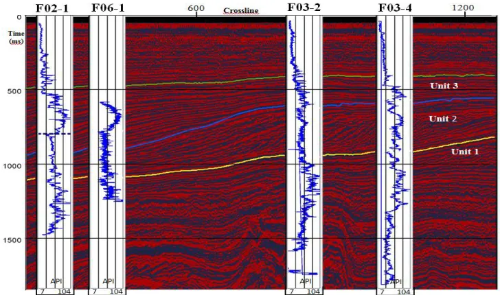
Fig. 2. The seismic section driven from original seismic data (in-line 425), showing the location of wells and presenting the gamma ray logs in every well

A basic rule for gamma ray log interpretation is that lower values correlate with sandy layers and higher values correlate with shaly layers [33]. According to this rule, the various shale and sand layers can be distinguished in Figure 2. Tetyukhina et al. [33] also interpreted the target zone by comparing the gamma ray log and P-wave velocity log. They applied a cross-plot of the gamma ray values against acoustic impedance values within the target zone to describe the target zone using the correlation between the two logs (Fig. 3b).

As shown in Figure 3a, the seismic cross-section is displayed in in-line 441, and well F03-4 whose location is illustrated in Figure 3a was selected to interpret various layers in the target zone using cross-plot analysis. ‘Truncation 1’ and ‘MFS4’ (white dashed lines) represent the position of the target zone interval in the seismic data. The cross-plot of the gamma ray values against acoustic impedance values, computed from the velocity and density logs, is presented in Figure 3b. The colour scale is assigned to the points as a function of depth to describe the correlation between the two logs. According to the results of Figures 2 and 3, two types of sediments can be distinguished in the target zone. Shale-rich sediments (600–750 m) with generally higher gamma ray values (>70 API) are depicted as

blue points, and sand-rich sediments (750–850 m) with generally low gamma ray values (<70 API) are shown as red points.

3.1. Pre -processing

In this research, the main objective is to correctly characterize the gas-bearing reservoir of F3 block in term of porosity using analysis of the attributes of seismic data. Seismic attributes could expose information which is not readily apparent in the raw seismic data. There are over 100 attributes which are applicable in some geophysical interpretation software packages [34], many of which result from slightly differing procedures to distinguish specific properties, such as amplitude or phase. An appropriate correlation between seismic attributes and porosity is seen often enough to convince us in the present work that the correlation is meaningful and that seismic attribute could be applied as an

agent for porosity in reservoir

(5)

177

Fig. 3. a) The seismic section (in-line 441) used for the cross-plot analysis [32]; b) A cross-plot of the gamma ray values against acoustic impedances values within the target zone [32]

Table 1. List of attributes used and their correlation coefficients with porosity values

Descriptive S tatistics

S tudied Attributes

Number of Points

Minimum Maximum Average S td. Deviation

Correlation Coefficient *S ig.

Porosity 927 0.221 0.344 0.286638 0.0236882 1

Energy 927 425250 16411000 4163775 3456700.9 -0.23 0.000

Envelope 927 139.5344 8602.5 2411.765 1748.5479 -0.26 0.000

Instantaneous Phase 927 -3.3283 3.1552 -0.191617 1.7112253 0.017 0.457

Instantaneous Frequency 927 -178.51 689.4833 209.9355 80.7153086 -0.101 0.000

Hilbert Transformation 927 -7365.5 6536.3 -36.39097 1992.0581 0.066 0.004

Amplitude 1st Derivative 927 -664760 548200 -3885.769 198827.97 -0.036 0.115

Amplitude 2nd Derivative 927 -111040000 126270000 -4254.58 34531237 -0.023 0.305

Cosine Phase 927 -1.0178 1.0477 -0.056109 0.6814381 -0.107 0.000

Envelope Weighted Phase 927 -3.0598 2.4849 -0.101663 1.0937449 -0.034 0.137

Envelope Weighted Frequency 927 -14.5334 305.4846 203.4539 51.1291469 -0.157 0.000

Phase Acceleration 927 -73638 64199 49.61784 12914.86 0.064 0.005

Thin Bed Indicator 927 -363.73 415.4329 6.48161 48.7964219 -0.002 0.918

Bandwidth 927 -0.5155 108.298 12.81416 11.9160097 -0.159 0.000

Q Factor 927 -5232.1 5676 -41.45138 398.0633953 -0.022 0.333

Instantaneous Rotate Phase 927 -6536.3 7365.5 36.39097 1992.0581 -0.066 0.004

Spectral Decomposition 927 304.8516 13142 4835.486 2861.6049 -0.307 0.000

Similarity 927 0.6861 0.9488 0.871362 0.0608897 -0.45 0.000

(6)

178 According to Table 1, the highlighted attributes are considered to be optimal ones to predict porosity as the output in linearity and non-linearity mode. In practice it is not too common to have correlation greater than 0.5-0.6 between seismic attributes and well log data, so this work is satisfied with using F3 data to find linear or non-linear relationships between two sets of input and output data. In this research, the candidate attributes such as energy, envelope, spectral decomposition and similarity are used to predict the spatial distribution of porosity in the North Sea reservoir using two different techniques. The first is an ANFIS algorithm which is implemented in three versions based on different clustering algorithms, and the second is an experimental model which is constructed using algebraic technique. Since the similarity is a fundamental attribute which shows more correlation than other attributes, the proposed model is introduced as an experimental equation between similarity attribute and porosity value to develop with the data set of the North Sea case; therefore it is known as a case-dependent model.

3.2. Adaptive neuro-fuzzy inference system (ANFIS)

ANFIS is a network structure consisting of a number of nodes connected through directional links. Each node is characterized by a node function with fixed or adjustable parameters. Once the fuzzy inference system is initialized, neural network algorithms can be used to determine the unknown parameters (premise and consequent parameters of the rules) and minimize the error measure, as conventionally defined for each variable of the system. Due to this optimization procedure, the system is described as adaptive. In fact, ANFIS is a fuzzy inference system; therefore it is necessary to initialize the FIS structure [35]. There are some methods to initialize the ANFIS structure before any parameter-tuning. For a given data set, different ANFIS models could be constructed using different identification methods. Clustering algorithms essentially deal with the task of partitioning a set of patterns into a number of homogeneous classes (clusters) with respect to a suitable similarity measurement. Clustering methods play an important role in the

areas of pattern recognition and classification. Several clustering algorithms are used to identify the antecedent parameters. The popular fuzzy c-means (FCM) and the Gustafson–Kessel (GK) clustering algorithms [36], the simplified Gustafson–Kessel (SGK) clustering algorithm [37], the Gath–Geva (GG) clustering algorithm [38], the simplified Gath–Geva (SGG) clustering algorithm [37], the modified Gath–Geva (MGG) clustering algorithm [39] and the subtractive clustering (SC) algorithm [40] have been used. Grid partitioning (GP), SCM and FCM are used in this paper to identify the antecedent membership functions. (Refer to Appendix A for further details on ANFIS structure.)

3.3. Implementation of ANFIS algorithms In order to implement ANFIS algorithms and train them with sufficient generality, the available data are divided into three subsets. The first subset is the training set, which is used to train the algorithms. The second subset is the validation set derived from training wells (F02-1, F06-1, F03-2). This set of data, which is not applied during the training, is used to validate the trained algorithms. The third subset is the testing set derived from testing well (F03-4); this well, which is not used during the training, is applied to obtain the overall accuracy of the algorithms and evaluate the generality of various ANFIS structures. ANFIS programming in MATLAB R2008a software is used here. To develop

ANFIS(GP), ANFIS(SCM) and

ANFIS(FCM), Genfis1, Genfis2 and Genfis3 commands are used, respectively. These commands generate initial structures of the Sugeno fuzzy inference system using grid partition, subtractive clustering and fuzzy c-means clustering algorithms, respectively. Figure 4 shows the fuzzy rule architecture of various developed ANFIS algorithms and Table 2 shows the details of ANFIS algorithms used in this study.

(7)

179

Table 2. The specification of ANFIS models developed by MATLAB

ANFIS Details ANFIS(GP) ANFIS(SCM) ANFIS(FCM)

Number of nodes: 55 117 67

Number of linear parameters: 80 55 30

Number of nonlinear parameters: 16 88 48

Total number of parameters: 96 143 78

Number of training data pairs: 1427 1427 1427

Number of fuzzy rules: 16 11 6

Fig. 4. Architecture of ANFIS , based on GP, S CM and FCM

(8)

180

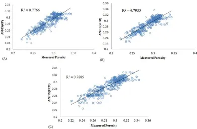
Fig. 6. Comparison of the measured and the predicted porosi ty of testing set: A) grid partition; B) subtractive clustering; C) fuzzy c-means clustering

For the learning process, the input vectors (energy, envelope, spectral decomposition and similarity) and corresponding target vectors (porosity) are used to train the ANFIS algorithms.

The validation and testing data set, which does not include any data from the training data set, is used to evaluate the generalization ability of ANFIS algorithms. Figures 5 and 6 illustrate the results of the three ANFIS algorithms based on the second and third sets. The comparison shows a slight superiority of ANFIS (SCM) over ANFIS(GP and FCM) in Figure 5. The R-square coefficient, which measures the strength of the linear relationship between the two variables (actual and predicted values), is R=0.7935. According to these results, it seems that the ANFIS algorithms could be a good method with which to estimate porosity distribution, while when the testing set is applied the same value decreased to 0.252. It is evident from these results that the generalization ability of ANFIS algorithms is not acceptable, and the predicted results do not match well with the experimental values.

(9)

181 more valid than single-attribute ones over the target zone. Improvements have focused on accuracy enhancement, shorter equations and improved representation of the sand and shale regions. Finally, in all these situations, various mixture models were developed that exhibit varied behaviour in contrast to sand and shale layers. The ultimate empirical function, which is a single-attribute equation based on the similarity attribute, is expressed as:

(1) s ln(s)

ln(s) c

Y  a b 

where Y denotes porosity and

s

is a similarity attribute. The coefficients of the equation (a, b and c) depend on the experimental data, and our investigations indicate that a limited set of data (sediments with gamma ray lower than 70 API) in the target zone could be used to adjust the coefficients. The deviations of porosity values calculated using this equation are much lower than those from the equation developed by sediments with gamma ray higher than 70 API.

The PFE is a non-linear function, and by substituting similarity into

s

porosity distribution could be estimated in the reservoir if the optimal constants (a, b, c) are in the pseudo-forward equation. Assuming that the PFE provides estimates of porosity values for different similarity attributes, at a particular depth under consideration, it could be applied to express a linear system of

n

linear equations with three unknowns as:

(2)

1 1 1 1

2 2 2 2

s ln(s ) 1 / ln(s ) 1

1 s ln(s ) 1 / ln(s )

N N N N

d a d b c d               _             _{  }    

The above equation is also a matrix equation which could be written symbolically as:

(3)

d = Gm

where G is the matrix of known coefficients, m is the unknown parameter vector containing (a, b, c), and d is the input data vector (similarity attribute from the seismic data at that particular depth). The matrix G is related to the geometry of the problem and not the data itself. Having more data than unknowns when

n



3

, the system of Equations 2 has no

exact solution. Jin et al. [41] showed that singular value decomposition (SVD) could be effectively employed for stabilization of inverse problems. The main advantage of SVD is that it provides a precise way of analysing a matrix, and yields a stable but approximate inverse. SVD is widely used in geophysical inversions, and in this work the SVD technique has been applied in the inverse problem.

3.5. SVD solution of PFE

Singular value decomposition (SVD) is a common and precise way of solving linear least squares problems [42]. For a general matrix G of order

n m



, which is a map from the model space to the data space, there is always a matrix decomposition called the singular value decomposition (SVD) of matrix G. Singular value decomposition allows the matrix G to be expressed as the product of three matrices [43]:

(4)

T

G UΛV

where Um m is the matrix of eigenvectors of

GGT that span the data space, and Vn n is the

matrix of eigenvectors of the G GT _{that span}

the model space. The singular values of the matrix G are the positive square roots of the eigenvalues of the matrix G GT . _{m n}_ is a matrix with the singular values of the matrix G in its main diagonal elements in a decreasing order. Menke [44] showed that the SVD of matrix G becomes

(5)

T T

P P P

G UΛV U Λ V

where the matrices UP and VP consist of the first p columns of U and V, related to non-zero singular values. _{p p}_ is a diagonal matrix with the non-zero singular values of the matrix G in diagonal elements. In the inversion calculations of the PFE equation 5 is applied, which is a reduced form of SVD. By the definition of the generalized inverse of a

matrix, the estimated solution vector mest will be obtained as:

(6) 1

V

est T

p p p

(10)

182 To get better model parameters for PFE, in this work we selected the sand data set (gamma ray < 70 API, N=268; P=3), consequently, the solution parameter vector mest is obtained from equation 6. The only potential difficulty in using SVD is when inverting a matrix that possesses some very small singular values (₁0.3020). If a singular value _j is small, the inverse of it becomes large and is dominated by numerical round-off error, which is undesirable. Menke [43] stated that when small singular values are excluded, the solution is generally close to the natural solution and possesses better variance. In this case,

10.3020

 which is small and near zero; therefore, the option is to arbitrarily set 10 so that p is reduced from 3 to 2, and

(7) 2 7.2697 0 0 181.1612 Λ _{ } _   (8) 2 0.9723 0.0815 0.2191 0.0072 0.0811 0.9966 V              (9) 2 0.0904 0.0245 0.0877 0.0257 0.0238 0.0560 U             

According to the abovementioned

equations, the optimized solution of PFE inverse problem could be written as:

(10) 1

2 2 2

est T

m  V U d

and

(11)

0.9723 0.0815

0.1376 0 0.0904 0.0877 0.0238 0.2191 0.0072

0 0.0055 0.0245 0.0257 0.0560 0.0811 0.9966 0.3003 0.3028 0.3008 0.0680 0.0019 0.3070 est m                    _{ } _{ } _                          

Based on the obtained solution, the final PFE model based on the sand data set of F3 block is implemented as:

(12)

0.0019 0.3028 0.0680 S ln(S)

ln(S)

Porosity   

Equation 12 is introduced as a data-driven mathematical model that is able to estimate the porosity distribution of a sandstone reservoir. To gain a better sense of the prediction power and generality of the optimized PFE, validation and testing sets were utilized that were similar to the ones employed in the ANFIS models.

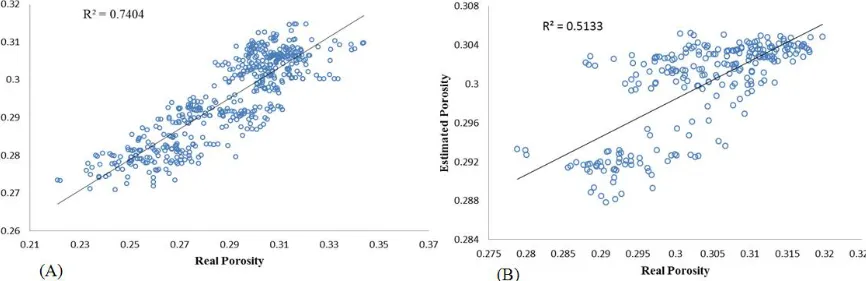
Figure 7 shows a scatter diagram of the observed values vs. the predicted outputs of the PFE model. From a comparison of the scatter plot of PFE and ANFIS models, the first thing to notice is that both developed models perform best with acceptable precision in the regions near to the training wells. As the testing data are exactly the same, this indicates

(11)

183 that the developed experimental model could better predict the porosity values of the regions far away from the training wells than the ANFIS algorithms. Therefore, there is a performance gap between training and testing locations that is considerable in ANFIS algorithms, while the proposed experimental model could reduce this gap.

3.6. Reservoir characterization using ANFIS and PFE

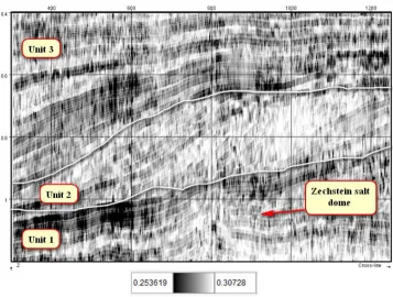
The interpretation of the target zone is fundamentally driven by the illustration of the spatial distribution of porosity predicted by the developed models. Figures 8 and 9 show the outputs of ANFIS algorithms (in-lines 244 and 442) and Figures 10a and 11 present the results of the PFE model in the same sections. In order to better differentiate the differences between the two models, a seismic line of porosity cube provided by dGB Earth Sciences Company is presented in Figure 10b, which is obtained via acoustic impedance inversion. In

Figure 10b it is evident that Unit 2 has more porosity value than other units (1 and 3) and does not exhibit any significant variations, except close to the red elliptical polygon associated with a vertical discontinuity, which is known as a gas chimney anomaly. The presence of gas chimneys has been interpreted as signifying hydrocarbon leakage pathways, and the mapping of such chimneys by neural network techniques has been established as an exploration tool. Wells drilled inside gas chimneys typically have higher pore fluid pressure, higher mud gas readings, higher mud gas wetness, more hydrocarbon shows, lower velocities, and higher temperatures than wells drilled outside gas chimneys [45]. Gas chimney and fault volumes extracted from 3D seismic data are rapidly becoming valuable tools for exploration and field development. In Figure 10a, the PFE model can detect this anomaly which marks the transition between the salt dome located in Unit 1 (Zechstein) and the near-surface gas pockets.

(12)

184

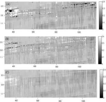
Fig. 9. The seismic sections of porosity (line 442) estimated by ANFIS : A) grid partition; B) subtractive clustering; C) fuzzy c-means clustering

(13)

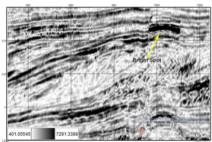
185 As indicated in Figure 11, the Zechstein salt dome is captured by the PFE model. It is clear that the feature of fault detection is driven by the similarity attribute. As in other researches, the similarity attribute map is applied to enhance the fault structures; furthermore, clear salt edges, and various seismic anomalies such as chimneys, faults, fractures, salt and sand bodies could be highlighted using the PFE technique that analyses data with combinations of similarity attributes. In addition to the patterns already defined in the PFE map, another anomaly could be found at about 530 ms in the map. In fact, F3 block contains a bright spot at about 530 ms possibly due to the presence of a gas packet. Chopra and Marfurt [46] demonstrate that reflections from gas-charged reservoir rocks showed much larger amplitudes than did reflections from adjacent oil or water saturated zones, and are often known as bright spots. A bright spot is obviously detectable in the instantaneous amplitude attribute, which is indicated with a yellow arrow in Figure 12. The instantaneous amplitude attribute of F3 block is illustrated in Figure 12. Additionally, in the output of the PFE model (Fig. 10a), the

bright spot is identified with a black arrow. On the other hand, when the outputs of ANFIS algorithms are considered (Figs. 8 and 9), it seems that there is a large gap between these results and the result reported by dGB Earth Science Company. A possible cause of inaccuracy in the ANFIS algorithms is the absence of enough available well data to provide sufficient generality in the trained models in the learning process. However, the inaccuracy could be seen in the PFE model with less intensity. Because the PFE model was developed only with the data set of sand sediments, it might be allowed to tune more appropriately to the sand units than the shale layers. In Figure 10a, this fact could be observed at the ‘A’ spot where there are deposits of shaly sediments. But, on the other hand, the opposite appears to be true at the ‘B’ spot where the model could estimate porosity distribution correctly. However, despite the few inaccuracies in the PFE results, the observations suggest that the PFE model has performed well within the gas-bearing sand reservoir of F3 block, and that ANFIS algorithms require a higher number of wells to develop with greater accuracy.

(14)

186

Fig. 12. The instantaneous amplitude attribute map (in-line 244): high amplitude in 530 ms is an indicator of the presence of charged gas.

Conclusion

1. This work developed a mathematical model and ANFIS algorithms to characterize the gas-bearing sand reservoir of F3 block in term of porosity.

2. The PFE model, which uses the similarity attribute for predicting the porosity values, has three unknown constants which are obtained using SVD method.

3. This article was not able to correlate the PFE on the shale data set; therefore this research concentrated on the behaviour of the PFE on the sand data set (sediments with gamma ray values > 70 API).

4. The point that is significant in the seismic sections obtained by PFE is its capability in enhancing the gas chimneys. The reason for this behaviour of PFE is that its intrinsic properties originate from the nature of similarity. The similarity attribute enhances the fault structures and salt edges.

5. Unit 2, which is known as one of the main gas reservoirs of the F3 block, shows higher porosity compared to the Units 1 and 3 using PFE.

6. According to the observations in the outputs of PFE, the ability to detect the geological structures such as faults (gas chimney), folds (salt dome) and bright spot, besides the porosity estimation of sandstone

reservoirs, could be used for a guideline in selecting the drilling points.

7. It should be stated that the implemented ANFIS algorithms could not estimate porosity of the North Sea reservoir acceptably, and did not capture the geological features observed in the well located in F3 block.

Acknowledgements

The manuscript benefited from the comments and suggestions given by the two referees of the International Journal of Mining and Geo-Engineering.

References

[1] Bhatt, A., Helle, H.B. (2002). Committee neural networks for porosity and permeability prediction from well logs, Geophysical Prospecting. 50, pp. 645–660.

[2] Anderson, J.K. (1996). Limitations of seismic inversion for porosity and pore fluid: Lessons from chalk reservoir characterization exploration, Society of Exploration Geophysicists, SEG Annual Meeting, Denver, Colorado, pp. 309-312.

(15)

187

methodology). The Leading Edge, 13, pp. 305-310.

[4] Lim, J.S. (2005). Reservoir properties determination using fuzzy logic and neural networks from well data in offshore Korea, Journal of Petroleum Science and Engineering, 49, pp. 182-192.

[5] Singh, V., Painuly, P. K., Srivastava, A. K., Tiwary, D. N., Chandra, M. (2007). Neural networks and their applications in lithostratigraphic interpretation of seismic data for reservoir characterization, 19th World Petroleum Congress, Madrid, Spain. pp. 1244-1260.

[6] Walls, J.D., et al., (2000). Seismic reservoir characterization of a U.S. Midcontinent fluvial system using rock physics, poststack seismic attributes, and neural networks, Society of Exploration Geophysicists , SEG Annual Meeting, Calgary, Alberta, pp. 428-436.

[7] Calderon, J. E., Castagna, J. (2007). Porosity and lithologic es timation using rock physics and multi-attribute transforms in Balcon Field, Colombia, The Leading Edge, 26(2), pp. 142-150.

[8] Joel, D. W., et al., (2002). Interpreter's Corner---Seismic reservoir characterization of a U.S. Midcontinent fluvial system us ing rock physics, poststack seismic attributes and neural networks, The Leading Edge, 21, pp. 428-436.

[9] Zhengping, L., Jiaqi, L.. (1998). Seismic-controlled nonlinear extrapolation of well parameters using neural networks, Geophysics, 63(6), pp. 2035-2041.

[10] Tonn, R. (2002). Neural network seismic reservoir characterization in a heavy oil reservoir, The Leading Edge, 21(3), pp. 309-312.

[11] Banchs, R. E., Michelena, R. J. (2002). From 3D seismic atrributes to pseudo-well-log volumes using neural networks: Practical considerations, The Leading Edge, 21(10), pp. 996-1001.

[12] Rafael, E. B., Reinaldo, J. M. (2002). From 3D seismic atrributes to pseudo-well-log volumes using neural networks: Practical

considerations, The Leading Edge, 21(10), pp.996-1001.

[13] Helle, H. B., Bhatt, A., Ursin, B. (2001). Porosity and permeability prediction from wireline logs using artificial neural networks: a North Sea case study ,Geophysical Prospecting, 49, pp. 431-444.

[14] Pramanik, A. G., et al. (2004). Estimation of effective porosity using geostatistics and multiattribute transforms: A case study, Geophysics, 69(2), pp. 352-372.

[15] Daniel, P. H., James, S. S., John, A. Q. (2001). Use of multiattribute transforms to predict log properties from seismic data, Geophysics, 66(1), pp. 220-236.

[16] Kevin, P. D., Curtis, A. L. (2004). Genetic-algorithm/neural-network approach to seismic attribute selection for well-log prediction. Geophysics, 69(1), pp. 212-221.

[17] Leiphart, D. J., Hart, B. S. (2001). Comparison of linear regression and a probabilistic neural network to predict porosity from 3-D seismic attributes in Lower Brushy Canyon channeled sandstones, southeast New Mexico, Geophysics, 66(5), pp.1349-1358.

[18] Russell, B., Hampson, D., Schuelke, J., Quirein, J. (1997). Multiattribute Seismic Analysis, The Leading Edge, 16, pp. 1439-1443.

[19] Adekanle, A., Enikanselu, P. A. (2013). Porosity Prediction from Seismic Inversion Properties over ‘XLD’ Field, Niger Delta, American Journal of Scientific and Industrial Research, 4(1), pp. 31-35.

[20] Lei, L., Wei, X., Shifan, Z., Zhonghong, W . (2011). Reservoir property prediction using the dynamic radial basis function network, Society of Exploration Geophysicists ,SEG San Antonio 2011 Annual Meeting, pp. 1754-1758.

(16)

188

[22] Hosseini, A., Ziaii, M., Kamkar Rouhani, A., Roshandel, A., Gholami, R., Hanachi, J. (2011). Artificial Intelligence for prediction of porosity from Seismic Attributes: Case study in the Persian Gulf, Iranian Journal of Earth Sciences, 3, pp.168-174.

[23] Basu, P., Verma, R. (2013). Multi attribute transform and Probabilistic neural network in effective porosity estimation-A case study from Nardipur Low area, Cambay Basin, India., 10th Biennial International Conference & Exposition, India, pp.131-139.

[24] Valenti, J. C. A. F., (2009). Porosity prediction from seismic data using multiattribute transformations, N Sand, Auger field, Gulf of Mexico, Ms.c Thesis, The Pennsylvania State University, The Graduate School.

[25] Joonaki, E., Ghanaatian, SH., Zargar, GH. (2013). An Intelligence Approach for Porosity and Permeability Prediction of Oil Reservoirs using Seismic Data, International Journal of Computer Applications, 80(8), pp. 19-26.

[26] Ziegler, P. A. (1990). Geological atlas of western and central Europe. Amsterdam: Elsevierfor Shell Internationale Petroleum Maatschappij, B.V.

[27] Van Boogaert, H. A. A., Kouwe, W. F. P. (1993). Nomenclature of the Tertiary of the Netherlands. RGD & NOGEPA. 50, The Netherlands, 2nd edition.

[28] Kay, C. (1993). The growth and gross morphology of Quaternary deltas in the southern North Sea. Ph.D. thesis, University of Edinborough.

[29] Steeghs, P., Overeem, I., Tigrek, S. (2000). Seismic volume attribute analysis of the Cenozoic succession in the L08 block (Southern North Sea): Global and Planetary Change, 27, pp. 245–262.

[30] Gregersen, U. (1997). Sequence stratigraphic analysis of Upper Cenozoic deposits in the North Sea based on conventional and 3-D seismic data and well-logs: Ph.D. thesis, University of Aarhus.

[31] Aminzadeh, F., & Groot, P.D. (2006). Neural networks and other soft computing techniques

with applications in the oil industry: EAGE.

[32] Tetyukhina, D., Luthi, S. M., Van Vliet, L. J., Wapenaar, K. (2008). High-resolution reservoir characterization by 2-D model-driven seismic Bayesian inversion: an example from a Tertiary deltaic clinoform system in the North Sea, Society of Exploration Geophysicists , SEG Las Vegas 2008 Annual Meeting, pp. 1880-1884.

[33] Luthi, S.M. (2001). Geological well logs: Their use in reservoir modeling: Springer-Verlag.

[34] Brown, A.R. (1999). Interpretation of Three-Dimensional Seismic Data, 5th edition: AAPG Memoir 42, SEG Investigations in Geophysics 9, Tulsa, Oklahoma, 514 p.

[35] Jang. J.R.S. (1999). ANFIS: adaptive-network-based fuzzy inference systems. IEEE Trans Syst, Man, Cybernet, 23(3), pp. 665–85.

[36] Gustafson, D., Kessel, W. (1979). Fuzzy clustering with a fuzzy covariance matrix, In: Proceedings of the IEEE CDC, San Diego, CA, USA, pp. 761–766.

[37] Hoppner, F., Klawonn, F., Kruse, R., Runkler, T. (1999). Fuzzy Cluster Analysis, Wiley, New York. 361p.

[38] Gath, I., Geva, A. (1989). Unsupervised optimal fuzzy clustering. IEEE Transactions on Systems, Man, and Cybernetics , 11, pp. 773– 781.

[39] Abonyi, J., Babuška, R., Szeifert, F. (2002). Modified Gath–Geva fuzzy clustering for identification of Takagi–Sugeno fuzzy models. IEEE Transactions on Systems, Man, and Cybernetics. Part B Cybern, 32, pp. 612–621.

[40] Chiu, S. L. (1994). Fuzzy model identification based on cluster estimation. Journal of Intelligent And Fuzzy Systems , 2, pp. 267–278.

(17)

189

[42] Sheriff, R.E. (1991). Encyclopedic Dictionary of Applied Geophysics, 4th Ed (Geophysical References).

[43] Lay, D.C. (1996). Linear algebra and its applications, 2nd ed, Addison-Wesley.

[44] Menke, W. (1989). Geophysical Data Analysis: Discrete Inverse Theory (Revised Edition), Academic Press.

[45] Løseth, H., Wensaas. L., Arntsen. B., Gading, M. (2008). Gas chimneys and other hydrocarbon leakage anomalies interpreted on seismic data, Internationa geological congress Oslo(Norway) 2008, August 6-14.

[46] Chopra, S., Marfurt, K.J. (2007). “Seismic attributes for prospect identification and reservoir characterization” Society of Exploration Geophysicists, Tulsa, 456 p.

[47] Lin, C. T., Lee, C. S. G. (1991). Neural-network-based fuzzy logic control and decision system. IEEE Trans Comput, 40(12), pp. 1320– 36.

(18)

190 Appendix A

A fuzzy inference system could model the qualitative aspects of human knowledge and reasoning processes without employing precise quantitative analyses. Neural networks (NN) are information-processing programs inspired by mammalian brain processes. NN are composed of a number of interconnected processing elements analogous to neurons. The training algorithm inputs to the NN a set

of input data and checks the NN output for the desired result. Combining neural networks with fuzzy logic has been shown to reasonably emulate the human process of expert decision-making. In traditional NN, only weight values change during learning, so that the learning ability of neural networks is combined with the inference mechanism of fuzzy logic for a neuro-fuzzy decision-making system [47].

Fig. 13. a) The first-order of TS K fuzzy model; b) corresponding ANFIS architecture (after [35])

Thus, an adaptive network is presented in Figure 13a which is functionally equivalent to the fuzzy inference system in Figure 13b. In the experiment, a neural fuzzy model is used [48] which consists of five layers:

Layer 1: Each node i in this layer generates a membership grade of a linguistic label. For instance, the node function of the ith node might be:

(1) 1 2 1 1 ( ) 1 i

i A i _b

i Q x x v   _ _ _     _  _      

where x is the input to node i, and A_i is the linguistic label (small, large, etc.) associated

with this node; and