DESIGN, SIMULATION AND MATHEMATICAL MODELLING OF THE DYNAMIC BEHAVIOR OF A VEHICLE TIRE AND CHASSIS SYSTEM AT A TURN

Http://www.ijetmr.com©International Journal of Engineering Technologies and Management Research [12]

DESIGN, SIMULATION AND MATHEMATICAL MODELLING OF THE

DYNAMIC BEHAVIOR OF A VEHICLE TIRE AND CHASSIS SYSTEM

AT A TURN

Mbelle Samuel Bisong *1, 2, 3, 4_{, Paune Felix} 5_{, Lokoue D. Romaric Brandon} 1_{, Pierre Kisito} Talla 2

1 _{ENSET Kumba, Cameroon}

2 _{LMMSP University of Dschang, Cameroon}

3 _{ENSET, University of Douala, Cameroon}

4 _{Ammosov’s North-Eastern FederalUniversity, 58 Belinskogo, 677000, Yakutsk, Russia}

5 _{Génie Informatique et Automatique, UFD-SCI, ENSET, University of Douala, Cameroon}

Abstract:

Road security has become with time a topic of concern in our society as per the increasing number of accidents and deaths occurring on the highways. Regulatory experts on road users have constantly been working for ways to solve this problem and thence better the lives of the citizens. This paper is aimed at proposing a mathematical model integrating specific parameters, describing the dynamic lateral behavior of a vehicle’s tire and chassis systems and enabling to state a relationship between road characteristics and vehicle dynamics. To achieve this, we made used of the fundamental theorems of dynamics for the modeling of the vehicle’s suspended and non-suspended masses and load transfers, then we associated this with the Pacejka Tire model to obtain a complete vehicle model. After the particularization of a global model, a simulator was realized named “DYNAUTO SIMULATOR” which iterates the given variables to produce a consistent result. After an experimental research made on the Ndokoti – PK 24 road section we could, thanks to our simulator determine the maximum speed to have at every turn of this road section and also understand the effect of the modification of a vehicle’s center of gravity on its stability. This work will be an important tool which can be recommended to the regulatory board as a major asset in the road construction policy and also in the improvement of road safety measures.

Keywords: Simulation; Modelling; Dynamic; Behavior; Vehicle; Road; Tire; Speed.

Cite This Article: Mbelle Samuel Bisong, Paune Felix, Lokoue D. Romaric Brandon, and Pierre Kisito Talla. (2020). “DESIGN, SIMULATION AND MATHEMATICAL MODELLING OF THE DYNAMIC BEHAVIOR OF A VEHICLE TIRE AND CHASSIS SYSTEM AT A TURN.” International Journal of Engineering Technologies and Management Research, 7(1), 12-23. DOI: 10.29121/ijetmr.v7.i1.2020.479.

1. Introduction

DOI: 10.29121/ijetmr.v7.i1.2020.479

Http://www.ijetmr.com©International Journal of Engineering Technologies and Management Research [13] vehicles each year are as facts as well. As a measure to palliate this dreadful phenomenon, the study of a vehicle’s behavior at a turn in order to illustrated all the risk has been conducted over the years by numerous engineers.

Our contribution to this is by basically designing a simulator which integrate the various vehicle, road and tire parameters and with the help of equations derived based on an analysis of vehicle’s lateral dynamics [1] iterate and calculate the vehicle’s specific speed at a particular turn on a road section.

A mathematical model is first of all designed from the fundamental theorems of dynamics and the variables which directly affect the Lateral dynamics of a vehicle which are the yaw speed and the center of gravity drift are sorted out and these will be the backbone of this software.

2. Materials and Methods

2.1.Materials

This work is centered on the programming of computer software and hence no physical material is required; all the tests were done in the computer and the various data were immediately implemented on the software. For this research paper, apart from the data collected from a research laboratory, the various materials were used such as:

1) DELL Latitude E6220 with 250GB HDD and 4GB RAM (Laptop). 2) The Analytical software MATLAB 2016 version.

2.2.Methods

2.2.1.Elaboration of the General Model

Before calculation and derivation of equations, it is important to set a foundation for these actions. Hence, we need to establish the reference frames which will be considered at any point in time. These frames are;

• The inertial frame (relates the vehicle trajectory to road surface) 𝑅₀(𝑂₀, 𝑥⃗⃗⃗⃗ , 𝑦₀ ⃗⃗⃗⃗ , 𝑧₀ ⃗⃗⃗ )₀

• The body frame (with respect to the suspended mass) 𝑅₁(𝐺, 𝑥⃗⃗⃗ , 𝑦₁ ⃗⃗⃗⃗ , 𝑧₁ ⃗⃗⃗ )₁

• The intermediary frame (with respect to the non-suspended mass) 𝑅₁₀(𝑀, 𝑥⃗⃗⃗⃗⃗⃗ , 𝑦₁₀ ⃗⃗⃗⃗⃗⃗ , 𝑧₁₀ ⃗⃗⃗⃗⃗ )₁₀

• The intermediary reference frame for rolling 𝑅₁₀̇ (𝑂₁, 𝑥⃗⃗⃗⃗⃗⃗ ₁₀∗, 𝑦⃗⃗⃗⃗⃗⃗ ₁₀∗, 𝑧⃗⃗⃗⃗⃗ ₁₀∗)

• The tires frame 𝑅𝑡(𝐵1, 𝑥⃗⃗⃗ , 𝑦𝑡 ⃗⃗⃗ , 𝑧𝑡 ⃗⃗⃗ )𝑡

The vehicle is basically a giant physical system and as such is subjected to the laws of Physics also known as Newton’s Laws.

𝛴𝐹

⃗⃗⃗⃗⃗ 0 _{= 𝑀𝛾}

𝐺0 (1)

Http://www.ijetmr.com©International Journal of Engineering Technologies and Management Research [14] While considering the first part, the forces acting at the reference points after being derived from (1), yield the following set of equations;

{ 𝑀 [𝑑𝑉

𝑑𝑡 − 𝛿𝑉(𝛿

.

+ 𝜓.)] = 𝐹𝑥𝑓𝐿+ 𝐹𝑥𝑓𝑅+ 𝐹𝑥𝑟𝐿+ 𝐹𝑥𝑟𝑅+ 𝑀𝑔 𝑠𝑖𝑛(𝛼0)

𝑀 [𝑉(𝛿. + 𝜓.) + 𝛿𝑑𝑉

𝑑𝑡] − 𝑀𝑠+ 𝜃 ..

= 𝐹_𝑦𝑓𝐿+ 𝐹_𝑦𝑓𝑅+ 𝐹_𝑦𝑟𝐿+ 𝐹_𝑦𝑟𝑅 𝑀𝑔 𝑐𝑜𝑠(𝛼₀) = 𝐹_𝑧𝑓𝐿+ 𝐹_𝑧𝑓𝑅+ 𝐹_𝑧𝑟𝐿+ 𝐹_𝑧𝑟𝑅

(3)

The Kinematic moment of the car body on G is obtained by supposing that the center of inertia of the car body is taken as the center of inertia of the whole vehicle and also that variation of the center of gravity’s position due to the wheels’ action is negligible. This is given by the expression:

𝜇_𝐺0 = 𝐼_𝑠𝑚𝛺⃗ ₁0

This expression is expanded and written as a matrix and hence the kinematic moment of the vehicle’s body on G is given by:

𝜇_𝐺0 = [ 𝐼𝑥𝑥𝑠𝑚𝜃 . + 𝐼𝑥𝑧𝑠𝑚𝜓 . 0 𝐼𝑥𝑧𝑠𝑚𝜃 . + 𝐼𝑧𝑧𝑠𝑚𝜓

.] (4)

The Kinematic moment of the 4 tires is obtained from determining the kinematic moment of one tire and then summing it to 4. The expression for the kinematic moment of one tire is derived from the expression below;

[𝜇_𝐵0_] 𝑖

𝑡𝑖𝑟𝑒 _{= 𝐼} 𝑖𝑡𝑖𝑟𝑒𝛺⃗ 𝑅𝑖

0

This expression is further expanded and written as a matrix so that the kinematic moment of one tire is represented by the equation;

[𝜇𝐵0]𝑖𝑡𝑖𝑟𝑒 = [ 0 𝐼𝑦𝑦𝑡𝑖𝑟𝑒𝜂𝑖

𝐼_𝑧𝑧𝑡𝑖𝑟𝑒𝜓. ]

10

Hence, summing the matrix above to the 4 tires, we get the expression for the kinematic moment of the 4 tires given as:

∑ [𝜇_𝐺0_] 𝑖 𝑡𝑖𝑟𝑒 4

𝑖=1 = [

0

∑ 𝐼_𝑦𝑦𝑡𝑖𝑟𝑒_𝜂 𝑖𝑗 4

𝑖𝑗=1

∑4𝑖=1(𝐼𝑧𝑧𝑡𝑖𝑟𝑒+ 𝑚𝑡𝑖𝑟𝑒(𝑎𝑖²+ 𝑏𝑖²))𝜓 .]

10

DOI: 10.29121/ijetmr.v7.i1.2020.479

Http://www.ijetmr.com©International Journal of Engineering Technologies and Management Research [15] The Kinematic moment of the axles is obtained in a similar manner as seen above with that of the 4 tires. Hence of summing the matrix of the kinematic moment of one axle to 4, we get the expression:

∑ [𝜇_𝐺0_] 𝑖 𝑎𝑥𝑙𝑒 4

𝑖=1 = [

0 0

∑4𝑖=1(𝐼𝑧𝑧𝑎𝑥𝑙𝑒+ 𝑚𝑎𝑥𝑙𝑒(𝑎𝑖²+ 𝑏𝑖²))𝜓 .]

10

(6)

Hence, the kinematic moment of the entire vehicle at the center of gravity, G which is the combination of the individual kinematic moments derived above is given by the expression;

𝜇_𝐺0 =

[ 𝐼𝑥𝑥𝑠𝑚𝜃 . + 𝐼𝑥𝑧𝑠𝑚𝜓 . ∑ 𝐼_𝑦𝑦𝑡𝑖𝑟𝑒𝜂_𝑖𝑗 4 𝑖𝑗=1 𝐼_𝑥𝑧𝑠𝑚𝜃. + 𝐼_𝑧𝑧𝑠𝑚𝜓. + ∑ (𝐼_𝑧𝑧𝑡𝑖𝑟𝑒+ 𝑚𝑡𝑖𝑟𝑒(𝑎_𝑖²+ 𝑏_𝑖²)) 4 𝑖=1 𝜓. + ∑(𝐼_𝑧𝑧𝑎𝑥𝑙𝑒+ 𝑚𝑎𝑥𝑙𝑒(𝑎_𝑖²+ 𝑏_𝑖²)) 4 𝑖=1 𝜓. ]₁₀

This kinematic moment is further simplified to get the expression;

𝜇_𝐺0 _{= [} 𝐼𝑥𝑥𝜃

.

+ 𝐼𝑥𝑧𝜓 .

∑4𝑖𝑗=1𝐼𝑦𝑦𝑡𝑖𝑟𝑒𝜂𝑖𝑗

𝐼_𝑥𝑧𝜃. + 𝐼_𝑧𝑧𝜓. ]

10

(7)

The dynamic moment of a system at a point is defined as the derivative of the kinematic moment of the system at that point. That is;

𝛤 _𝐺0 =𝑑

0

𝑑𝑡𝜇 𝐺

0

Hence, the dynamic moment of the vehicle at the point G is given by the expression;

𝛤 _𝐺0 = [

𝐼_𝑥𝑥𝜃.. + 𝐼_𝑥𝑧𝜓.. − ∑4_𝑖𝑗=1𝐼_𝑦𝑦𝑡𝑖𝑟𝑒𝜂_𝑖𝑗𝜓.

−𝐼𝑥𝑥𝜃 .

𝜓. − 𝐼𝑥𝑧𝜓2 .

+ ∑4𝑖𝑗=1𝐼𝑦𝑦𝑡𝑖𝑟𝑒𝜂𝑖𝑗

𝐼_𝑥𝑧𝜃.. + 𝐼_𝑧𝑧𝜓..

]

10

(8)

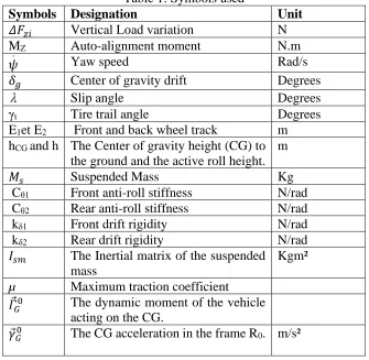
Http://www.ijetmr.com©International Journal of Engineering Technologies and Management Research [16] Table 1: Symbols used

Symbols Designation Unit

𝛥𝐹_𝑧𝑖 Vertical Load variation N

MZ Auto-alignment moment N.m

𝜓. Yaw speed Rad/s

𝛿_𝑔 Center of gravity drift Degrees

 Slip angle Degrees

γt Tire trail angle Degrees

E1et E2 Front and back wheel track m

hCG and h The Center of gravity height (CG) to

the ground and the active roll height. m

𝑀_𝑠 Suspended Mass Kg

Cθ1 Front anti-roll stiffness N/rad

Cθ2 Rear anti-roll stiffness N/rad

kδ1 Front drift rigidity N/rad

kδ2 Rear drift rigidity N/rad

𝐼𝑠𝑚 The Inertial matrix of the suspended mass

Kgm²

µ Maximum traction coefficient 𝛤 _𝐺0 The dynamic moment of the vehicle

acting on the CG.

𝛾 _𝐺0 The CG acceleration in the frame R0. m/s²

The next step is determining expression for the vertical loads of the axles which are the front and rear axles, the values for these loads greatly influence derivability. These expressions are given below in terms of the transversal acceleration;

At the Front axle;

𝛥𝐹_𝑧𝑓 =𝑀𝑓ℎ1+𝑀ℎ( 𝐶𝜃1

𝐶𝜃)𝜃

𝐸1 𝛾𝑡 (9)

At the rear axle;

𝛥𝐹_𝑧𝑟= 𝑀𝑟ℎ2+𝑀ℎ( 𝐶𝜃2

𝐶𝜃)𝜃

𝐸2 𝛾𝑡 (10)

Finally, determining these vertical loads at each of the tires is important in the understanding of the vehicle’s dynamic behavior. This is an accurate interpretation of the Pacejka model [16] as it clearly illustrates the tire/road relationship. Hence for each of the tires, their vertical loads are;

Front left tire: 𝐹_𝑧𝑓𝐿=1

2𝑀𝑓𝑔 𝑐𝑜𝑠 𝛼0 − 1

𝐸1(𝑀𝑓ℎ1+ 𝑀ℎ 𝐶𝜃1

𝐶𝜃 + 𝐴𝜃1𝜃 .

DOI: 10.29121/ijetmr.v7.i1.2020.479

Http://www.ijetmr.com©International Journal of Engineering Technologies and Management Research [17] Front right tire: 𝐹𝑧𝑓𝑅=

1

2𝑀𝑓𝑔 𝑐𝑜𝑠 𝛼0+ 1

𝐸1(𝑀𝑓ℎ1+ 𝑀ℎ 𝐶𝜃1

𝐶𝜃 + 𝐴𝜃1𝜃 .

) (𝛾𝑡𝑐𝑜𝑠 𝜆 − 𝑔 𝑠𝑖𝑛 𝜆) (12)

Rear left tire: 𝐹_𝑧𝑟𝐿 =1

2𝑀𝑟𝑔 𝑐𝑜𝑠 𝛼0− 1

𝐸2(𝑀𝑟ℎ2 + 𝑀ℎ 𝐶𝜃1

𝐶𝜃 + 𝐴𝜃2𝜃 .

) (𝛾_𝑡𝑐𝑜𝑠 𝜆 − 𝑔 𝑠𝑖𝑛 𝜆) (13)

Rear right tire: 𝐹_𝑧𝑟𝑅= 1

2𝑀𝑟𝑔 𝑐𝑜𝑠 𝛼0+ 1

𝐸2(𝑀𝑟ℎ2+ 𝑀ℎ 𝐶𝜃1

𝐶𝜃 + 𝐴𝜃2𝜃 .

) (𝛾_𝑡𝑐𝑜𝑠 𝜆 − 𝑔 𝑠𝑖𝑛 𝜆) (14)

2.2.2.Elaboration of a Particular Model

This model is based on the general model above with the only particularity that it is centered only on the movement of the vehicle in the lateral plane (lateral dynamics). Studying lateral dynamics implies that the moment will only be considered in the x and z directions of the plane. That is;

Along x;

(𝐼_𝑥𝑥+ 𝑀_𝑠ℎ2)𝜃.. + 𝐼_𝑥𝑧𝜓.. − 𝑀ℎ (𝑉(𝛿. + 𝜓.) + 𝛿𝑑𝑉

𝑑𝑡) = 𝑀𝜃1(𝜃) + 𝑀𝜃 . 1(𝜃 . ) + 𝑀_𝑔(𝜃) Along z; 𝐼_𝑥𝑧𝜃.. + 𝐼_𝑧𝑧𝜓.. + 𝑀ℎ𝜃𝑑𝑉

𝑑𝑡 = 𝐿1(𝐹𝑦𝑓𝐿+ 𝐹𝑦𝑓𝑅) − 𝐿2(𝐹𝑦𝑟𝐿+ 𝐹𝑦𝑟𝑅)

In this case, the vehicle speed is a constant because the longitudinal dynamics is not considered. Hence for this model only the yaw speed and center of gravity drift equations from the general model equations;

𝑀𝑉(𝛿. + 𝜓.) = 𝐹𝑦𝑓𝐿+ 𝐹𝑦𝑓𝑅 + 𝐹𝑦𝑟𝐿+ 𝐹𝑦𝑟𝑅 (15)

𝐼_𝑧𝑧𝜓.. = 𝐿₁(𝐹_𝑦𝑟𝐿+ 𝐹_𝑦𝑓𝑅) − 𝐿₂(𝐹_𝑦𝑟𝐿+ 𝐹_𝑦𝑟𝑅) (16)

In this study, we introduced the drift coefficient which is the linear relation between the transversal force and the drift angle of the vehicle. It is hence given by;

𝐹_𝑦𝑖(𝛿_𝑖) = −𝑘_𝛿𝑖𝛿_𝑖 (17)

The drift coefficient after being substituted into the two equations (15) and (16) above will modify them into;

𝑀𝑉(𝛿.(𝑡) + 𝜓.(𝑡)) = −2𝑘_𝛿1(𝛿(𝑡) +𝐿1 𝑉 𝜓

.

(𝑡) − 𝜀_𝑟(𝑡)) − 2𝑘_𝛿2(𝛿(𝑡) −𝐿2 𝑉 𝜓

.

(𝑡)) (18)

And

𝐼_𝑧𝑧𝜓..(𝑡) = −2𝐿₁𝑘_𝛿1(𝛿(𝑡) +𝐿1 𝑉 𝜓

.

(𝑡) − 𝜀_𝑟(𝑡)) + 2𝐿₂𝑘_𝛿2(𝛿(𝑡) −𝐿2 𝑉 𝜓

.

Http://www.ijetmr.com©International Journal of Engineering Technologies and Management Research [18] In order to determine the expression for the yaw speed equation (19) is reduced and solved as a differential equation of second order. Hence, we get the expression of the yaw speed of a vehicle in a stabilized mode as;

𝜓.(𝑡) = 𝑉𝐿1𝑘𝛿1

(𝐿12𝑘𝛿1+𝐿22𝑘𝛿2)[1 − exp (−

2(𝐿12𝑘𝛿1+𝐿22𝑘𝛿2)𝑡 𝑉𝐼𝑍𝑍 )]

𝜋

180εr (20)

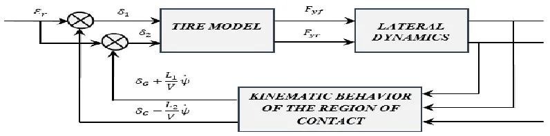
A block representation of this model is setup to illustrate the inputs, every parameter in play as well as the outputs which in this case are the yaw speed and the center of gravity drift.

Figure 1: Block representation of the Dynamic model.

The Center of gravity drift is obtained in the same manner as the yaw speed gotten above. That is, reducing the equation to a differential equation and then solving it to get its expression.

𝛿𝑔(𝑡) = −(𝛼 + 𝐾)exp (−

2(𝑘𝛿1+𝑘𝛿2)

𝑀𝑉 𝑡) + 𝐾exp (−

2(𝐿12𝑘𝛿1+𝐿22𝑘𝛿2)

𝑉𝐼𝑧𝑧 𝑡) + 𝛼 (21)

In addition to these two important variables which basically make up the core of our model, we introduced a variable which is often considered a factor of stability of a vehicle and it is called the Over steering rate. This rate is closely related to whether the vehicle is over steering or under steering. It is given by the expression;

𝑅_𝑂𝑆 = (𝑑𝜀𝑠(𝛾𝑡) 𝑑𝛾𝑡 ) =

𝑀𝑓 𝑘𝛿1−

𝑀𝑟

𝑘𝛿2 (22)

2.2.3.Simulation of the Model

DOI: 10.29121/ijetmr.v7.i1.2020.479

Http://www.ijetmr.com©International Journal of Engineering Technologies and Management Research [19]

Tire Characteristics

Brand and type; Michelin 245/45R18-100WO.1 Tire trail; 0.025m

Road Section Characteristics Slope; 7°

Transversal Slope; 2.5° Curvature radius; 70m

3. Results and Discussion

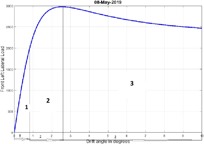
Figure 2: The Graph illustrating Lateral Load vs Drift angle for the front tire.

This curve is generated by the simulator, divided in three zones.

Zone 1: Represents the Tire adherence zone. Here the tire adheres to the road, the more the drift angle increases, the more the transversal effort generated by the tire increases.

Zone 2: Represents the Transition zone where the tire starts to slip. The curve increases in a non-linear manner before reaching a maximum point also known as saturation. Even as the drift angle increases, the transversal effort does not increase anymore.

Zone 3: Represents the slip zone where the tire has completely lost adherence. Here, the transversal effort decreases as the drift angle increases. There is tire slip; meaning a loss in derivability as the vehicle can’t go on the wanted trajectory. If the driver increases the steering angle and thus the wheel camber, he increases the drift angle and consequently decreases the transversal effort generated by the tire.

1 2

Http://www.ijetmr.com©International Journal of Engineering Technologies and Management Research [20] Figure 3: The Graph illustrating auto-alignment moment vs the drift angle for the front left tire. This curve reaches a maximum then decreases abruptly till the auto-alignment moment reaches

zero. If the drift angle keeps increasing, the auto-alignment sign changes to negative.

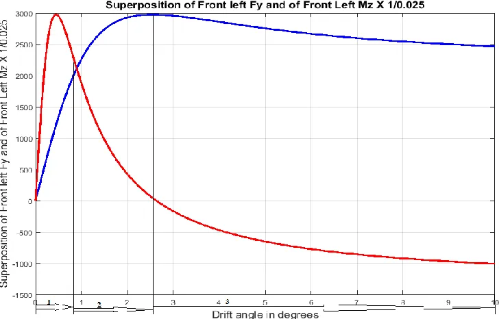
Figure 4: Superposition of lateral load to drift angle and auto-alignment moment to drift angle.

This superposition graph is generated by the simulator in order for the user to study and compare the evolution of both properties. It is also divided in three zones;

DOI: 10.29121/ijetmr.v7.i1.2020.479

Http://www.ijetmr.com©International Journal of Engineering Technologies and Management Research [21] In the first zone, we have a simultaneous increase of the auto-alignment moment Mz and the lateral

load Fy with respect to the drift angle. The superposition of these curves enables us to note that Mz

reaches its maximum before Fy. The fall in Mz is related to the tire entry into the transition zone.

Figure 5: Vehicle’s yaw speed with respect to time.

This yaw speed is specific for the vehicle’s steering angle (30° in this case) and is an essential property in the study of the vehicle lateral dynamics.

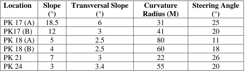
Http://www.ijetmr.com©International Journal of Engineering Technologies and Management Research [22] The simulator is hence used to iterate the vehicle’s speed on the chosen road section in order to determine the specific speed to have at a turn in that section. The table below illustrates the road parameters collected at the various turn on the Ndokoti – PK24 road section;

Table 2: Road data

Location Slope

(°)

Transversal Slope (°)

Curvature Radius (M)

Steering Angle (°)

PK 17 (A) 18.5 6 31 25

PK17 (B) 12 3 41 20

PK 18 (A) 5 2.5 80 11

PK 18 (B) 4 2.5 60 18

PK 21 7 3 22 26

PK 24 3 3.4 55 20

As said earlier, this procedure works for any brand-new car and any type of passengers’ vehicle, as long as the user has all the necessary information concerning this vehicle and the type of tire used. It should be noted that a modification in a vehicle’s center of gravity affects its lateral dynamic behavior and hence the speed values are not the same. In this case, the new center of gravity height should be introduced, and the iterations made again to get the new values for the modified vehicle.

4. Conclusion

The constant road accidents leading to severe loss of lives and properties has prompted the research of this article which deals with studying the dynamic behavior of a vehicle’s tire and chassis systems at a turn with the focus on determining the specific maximum speed that a particular vehicle should have at a particular turn on a road section. Modelling the vehicle’s dynamic behavior from its basic structural characteristics also reveals how this behavior can be influenced by a modification applied in the vehicle’s structure. The simulator which takes into consideration all the various aspects of a vehicle’s dynamics appears to be an essential tool in the fight against road accidents and thus the betterment of the lives of all road users in general.

References

[1] M. Mondek, M. Hromčik (June 2017); Linear analysis of Lateral vehicle Dynamics; Internal

Conference on Process Control.

[2] S. Jadhao, M.K Patil (2017); Modelling and Simulation of Full vehicle to study its dynamic

behavior; IJEDR.

[3] A. Express; Modelling of Automotive Systems: Lateral Vehicle Dynamics; University of Sussex.

[4] G. Gim, P. Nikravesh (1990); An Analytical model of pneumatic tyres for vehicle dynamic

simulations: Part One; Pure slips (vol 11 pp 589 – 618); International Journal of vehicle design.

[5] J.P Brossard (2006); Dynamique du Véhicule: Modélisation des systèmes complexes; Presses

polytechniques et universitaires romandes.

[6] S.E Kingue (2002); Cours de Dynamique du solide; Université du Douala; non-publié.

[7] J.P Timba (2014); Conception et design de l’automobile (cours); Enset de Douala; non-publié.

DOI: 10.29121/ijetmr.v7.i1.2020.479

Http://www.ijetmr.com©International Journal of Engineering Technologies and Management Research [23]

[9] D. Houcque (August 2005); Introduction to MATLAB for Engineering students; Northwestern

University.

[10] J. Kiefer (August 1996); Modelling of road vehicle lateral dynamics; RIT Scholar Works.

[11] J. Van Ginkel (July 2014); Estimating the Tire-Road Friction Coefficient based on Tire Force

Measurements; Delft University of Technology.

[12] D. Westbom, P. Frejinger (November 2002); Yaw control using rear wheel steering; Tekniska

Högskolan i Linköping.

[13] C. Ferreira, A. Netsunajev (February 2011); Programming with MATLAB; EUI.

[14] P. Polack, F. Altché, B. D’Andréa-Novel, A. De La Fortelle (June 2017); The Kinematic

Bicycle Model: A Consistent Model for Planning Feasible Trajectories for Autonomous Vehicles; IEEE Intelligent Vehicles Symposium (IV).

[15] H. Pacejka, E. Bakker, L. Nyborg; Tyre modelling for use in vehicle dynamics studies; SAE Paper

No. 870421

[16] H.B. Pacejka (2006); Tire and Vehicle Dynamics; Second Edition; Elsevier,

Butterworth-Heinemann.

[17] Bin Wang (2013); State observer for diagnosis of dynamic behavior of vehicle in its environment;

Université de Technologie de Compiègne.

[18] Georg Rill (August 2007); Vehicle Dynamics; University of Applied Sciences; Brazil.

[19] Huei Peng (2014); Vehicle Dynamics (ME542); University of Michigan.

[20] B. Jacobson et al (2016); Vehicle Dynamics (course) ; Chalmers University of Technology.

[21] K. Reif (2014); Brakes, Brake Control and Driver Assistance systems; Bosch Professional

Automotive Information.

[22] R. Di Martino (2005); Modelling and Simulation of the Dynamic Behavior of the Automobile;

Universite de Haute – Alsace Mullhouse.

[23] M.T VU (2012); Vehicle steering Dynamic Calculation and Simulation; DAAAM International.

[24] R.T Uil (2007); Tyre Models for steady-state vehicle handling analysis; Eindhoven University of

Technology.

[25] P.F.H Dugoff and L. Segel (1970); An analysis of tire traction properties and their influence on

vehicle dynamic performance (Vol 3 pp 1219 – 1243); SAE Transaction.

[26] V. Van Geffen (2009); A study of Friction models and friction compensation; Eindhoven

University of Technology.