BAYESIAN CLASSIFICATION OF HIGH DIMENSIONAL DATA
WITH GAUSSIAN PROCESS USING DIFFERENT KERNELS
Oloyede I.
Department of Statistics, University of Ilorin, Ilorin, Nigeria
Corresponding Author: Oloyede I., [email protected] ABSTRACT: The study investigates asymptotic
classification of high dimensional data by adopting Gaussian Process, five different kernels(covariance functions) were employed and compared to showcase the outperformed kernel asymptotically. Log marginal likelihood, Accuracy and log loss were the measurement criteria adopted to measure classification performances. The study therefore observed that the classification performed well asymptotically and found out that Gaussian Process Maximum Likelihood(GPML) had overall best model improvement asymptotically and across the covariance structures. K3 and K4 had the best accuracy in classification paradigm at the lower sample sizes but GPML and learned kernel had best model accuracy as the sample sizes tend to large sizes.
KEYWORDS: Bayesian, Kernels, Classification and Gaussian Process.
1. INTRODUCTION
Gaussian processes attempt to use mean and covariance function in lieu of mean and covariance used in Gaussian distribution. Though support vector machine is a celebrated classifier (SVM), it is not specifically designed to select features relevant to the predictor. In genetic research with thirty-five patients, if each patient has 178000 genes out of which only 32 genes may be relevant to the specific ailment that those patients are suffering from. The SVM cannot in anyway select those genes for classification since it does not have automatic relevance detection (ARD) which had been built specifically into Bayesian Gaussian processes. In network intrusion, there is need to have relevant information for the network defense. Bayesian learning algorithm is built with Automatic Relevant Determination that is able to predict the posterior probability ([Olo17]).
Gaussian processes are the prior distribution for regression and classification models where they are not limited to only simple parametric form. It is affirmed that Gaussian process had variety of covariance function with which it can be chosen from for different degree of smoothness. In this study four different classes of kernels are adopted.
GP proved to be the easiest way for classification though in a Bayesian paradigm where there is need to integrate over posterior density for the hyperparameter of the covariance function ([Rad98]).
Yi et al ([YSC11]) claimed that GP classification is best fit high dimensional covariates compared with other non-parametric approaches that can only model one to two dimensional covariates. GP has Automatic Relevance Determination (ARD) which takes care of the irrelevant features by removing them for the model whenever the covariance structure is irrelevant to the features input. They proposed penalized regression approach to the Gaussian process regression model where they opined that dealing with high dimensional data often resulted in large variances of parameter estimation and high predictive errors. Shi et al ([SMT03]) examined Bayesian regression and classification by mixing Gaussian Process, their study concluded that Bayesian approach leads to robust models as compared with optimization approach.
Kemmler et al ([K+13]) considered homoscedastic Gaussian noise in their experiment of one-class classification Gaussian process and concluded that the Gaussian process based measures is suitable for regression and classification of novelty detection problems.
In Bayesian classification paradigm, Gaussian prior is adopted since the marginal and conditional posteriors are normal, this is advantageous over other distribution ([Fon17]). The Gaussian process can be regarded as distribution over function and is fully specified as . Both the mean and covariance function of the GP can be
expressed as ;
. The GP
involves the covariance function and its hyperparameter. There will be no need to adopt complicated mean function ([Fon17]).
Bayesian treatment. Williams and Rasmussen ([WR86]) claimed that GP prior application over function outperformed other state of the art method of classification. Shi et al ([SMT03]) claimed that Bayesian learning using GP priors elicit knowledge from covariance based kernel parameter with ex ante information (prior belief) that yield posterior density with respect to training datasets. Kaiguang et al ([KPX00]) compared GPC model with k-nearest neighbor and support vector machine then concluded that GPC outperformed KNN and SVM thus yielded classification accuracy.
By and large, most of the renown authors working on GP had not examined asymptotic behaviour both at lower and high dimensional data subject to some redundancy, this is the gap this study is try to fill. Kemmler ([K+13]) claimed that machine learning conjugated with Gaussian prior gave room for the formulation of kernel based learning algorithm in a Bayesian paradigm. They derived one-class classification approach which is based on kernel based algorithm of Bayesian framework. They claimed that their one class classification approach outperformed the well-known support vector data description, this may be due to the presence of Automatic Relevance Determination (ARD) which is embedded in Gaussian process. In pattern recognition, it is main goal is to classifying the data in to c regions with the decision boundaries as the boundaries between the regions. It has been opined in the literature that the optimum classification is based on the use of posterior probability of class membership ([AS06]). The supervised learning algorithm usually predict outcomes(y) given a new set of predictor(X) - testing datasets which is totally different from the training datasets D that is used to fit the model ([Fon17]). In lieu of the above scenario, Gaussian Process adopted posterior predictive distribution which is probabilistic with mean and covariance functions.
2. METHODOLOGY
Let the input pattern x be assigned to one of C classes . Probabilistic classification is adopted in the study where test predictive is of the form of class probability rather than guessing of the class label. Let be the joint probability where y denotes the class label. The generative approach(sampling paradigm) models the class-conditional distribution for with the prior probability for each class
(2.1)
Discriminative approach (diagnostic approach) models . Due to hard problem that usually resulted from the density estimation of the class conditional distribution, the generative approach may be chosen. It could be established that discriminative approach can model directly but failed in an attempt to proffer solution to overfitting and hard problems of Rasmussen and Williams ([RW06])
(2.2)
The case of multi-class GP classification models is observed where t=-1, 0 or 1 to label three distinctive classes of latent target variable; often denoted by
. The input vector of n-dimensional features is denoted by x-covariates as .The feature variables were generated by uniform distribution with 25 redundant variables.
Given a set of training data
1,.., ; =0,1,2 with input ∗ dimension and target value, with a fixed hyperparameter. In GP classification there are possibility of selecting covariance prior from sets of covariance available.
( )2+ 1 (2.3)
where as the hyperparameters.
For multi class where target variable has characteristic of three or more categories form the set [0,1,…,k] . The k latent variable is defined as
(2.4)
where Gaussian process.
The class of a large training set is denoted as with a different value of features and the class conditional probability is expressed as for feature vector x. the Bayes theorem based on one classification is
. (2.5) Thus is the likelihood( class conditional probability) which is expressed with Gaussian Distribution(this uses mean and covariance),
posterior probability for each of the classes and thereafter select the one with the larger posterior.
Under the high dimensional features, the Gaussian Distribution is
∗ (2.6) Then the class –conditional probability is
∗ (2.7)
The expression can be regarded as mehalonobis distance as similar to
.
Let where
be the regressors or features and e is the disturbance term with zero mean and covariance function. Considering the expectation:
(2.8)
(2.9)
thus by adopting the Gaussian Process and the covariance function.
This is obtainable after the model had been fitted as
∗ ∗ ∗ ∗ ∗ ∗ (2.10)
Thus posterior mean is obtained as
∗ ∗ ∗ (2.11)
∗ ∗ ∗ ∗
2 −1 ∗, (2.12)
The covariance function is expressed as ∗ adopting the single feature vector xi with we have . Thus the study imposed redundancy in the data generation process. This is therefore affected the covariance function thereby corrupting the variances, we have where .
Exponential Squared Kernel: this is the setting of the
element of the covariance matrix for the univariate feature vector:
. The prior indicates that and are less correlated with reference to the distance between and .
Linear kernel let x and y be on the basis function such that
The target vector is drawn from multinomial distribution of the set classes and the feature
drawn from uniform distribution that is contaminated with some redundant input, it should be noted that Bayesian classification with Gaussian process has Automatic Relevance Detection (ARD) that can identify the relevant input for classification using the transfer function of multinomial logistic function. We define the multi-class problem as
with the hyperparameter v assigned with Gaussian priors as
.
The mean function is attributed with while the implies covariance function is of the various Kernels such as
(2.13) is the jitter that is added to improve the efficiency of the sample ([SMT03]).
Classification Problems:
3. RESULTS
Gaussian prior conjugated with likelihood choosing different covariance structure, five different covariance functions were adopted out of which two were combination of four covariance function. 1000 features (high dimensional data) with the sample sizes: 26; 54; 100; 200; 500 and 1000, 1000 features were generated and infused with multicollinearity, the study specified 20 redundant features with three clases of dependent variables, 2 classes per cluster. We used K1 to capture a long term, smooth rising trend with RBF kernel with a large length-scale enforces the component to be smooth. K2 was used to capture a seasonal component of periodic ExpSineSquared kernel with a fixed periodicity of 1 year. The length-scale of this periodic component, controlling its smoothness, is a free parameter. K3 was adopted to captured smaller, medium term
irregularities of RationalQuadratic kernel
which determines the diffuseness of the length-scales, are to be determined whereas K4 captured a “noise” term, consisting of an RBF kernel contribution of the correlated noise components such as local weather phenomena, and a WhiteKernel contribution for the white noise. We therefore sum up the four covariance functions with different parameters to derive Gaussian process maximum likelihood(GPML) and learned kernels.
Table 3.1. The asymptotic Gaussian Process classification using GPML covariance function for
high dimension data
Sample size
LML Accuracy Log-loss 26 -18.463 0.167 1.111
GPML 54 -37.292 0.455 1.086
100 -68.243 0.7 1.056
200 -125.489 0.4 1.081 500 -306.332 0.46 1.058 1000 -603.144 0.52 1.032 Table 3.1 showed the asymptotic classification of high dimensional data with GPML kernel. It was observed that as the sample size increases from 26 to 1000 the model improved with decrease in negative log likelihood from -18.46 to -603.14, thus obeyed law of large number. The study observed the accuracy and precision of the classification as the sample as the sample size increases from 26 to 100 with increased in accuracy from 0.17 to 0.7 at sample size 100 but it upturned when the sample size increased to 200, the study revealed that the accuracy got increased as the sample size increased from 200 up till 1000. The log loss improved strategically from sample sizes from 26 to 100 as it decreased from 1.11 to 1.06 but upturned as the sample size increased to 200, thereafter improved as the sample size increased from 200 up to 1000.
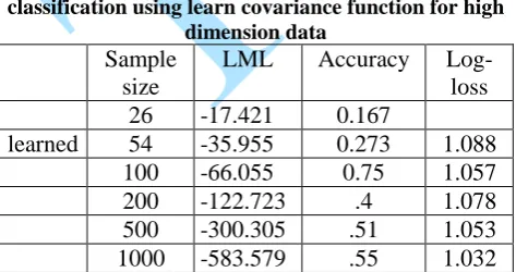
Table 3.2. The asymptotic Gaussian Process classification using learn covariance function for high
dimension data
Sample size
LML Accuracy Log-loss 26 -17.421 0.167
learned 54 -35.955 0.273 1.088 100 -66.055 0.75 1.057
200 -122.723 .4 1.078
500 -300.305 .51 1.053 1000 -583.579 .55 1.032 Table 3.2 showed the asymptotic classification of high dimensional data with learned kernel. It was observed that as the sample size increases from 26 to 1000 the model improved with decrease in negative log likelihood from -17.421 to -583.579, thus
obeyed law of large number. The study observed in the accuracy and precision of the classification, as the sample size increases from 26 to 100, the accuracy increased from 0.167 to 0.75 but it upturned when the sample size increased to 200, the study revealed that the accuracy got increased as the sample size increased from 200 up till 1000. The log loss improved strategically from sample sizes 26 to 100 as it decreased from 0 to 1.057 but upturned as the sample size increased to 200, thereafter improved as the sample size increased from 200 up to 1000 it decreases from 1.078 to 1.032.
Table 3.3. The asymptotic Gaussian Process classification using GPML covariance function for
high dimension data
Sample size
LML Accuracy Log-loss
26 -18.359 .167
54 -37.265 .455 1.086
K1 100 -68.224 .7 1.086
200 -125.406 .375 1.081
500 -306.19 .44 1.058
1000 -603.933 .53 1.029
Table 3.3 showed the asymptotic classification of high dimensional data with learned kernel. It was observed that as the sample size increases from 26 to 1000 the model improved with decrease in negative log likelihood from -18.359 to -603.933, thus obeyed law of large number. The study observed in the accuracy and precision of the classification, as the sample size increases from 26 to 100, the accuracy increased from 0.17 to 0.7 but it upturned when the sample size increased to 200, the study revealed that the accuracy got increased as the sample size increased from 200 up till 1000. The log loss improved strategically from sample sizes 26 to 1000 as it decreased from 1.086 to 1.029.
Table 3.4. The asymptotic Gaussian Process classification using GPML covariance function for
high dimension data
Sample size
LML Accuracy Log-loss 26 -13.873 0.333 1.099 54 -29.853 0.091 1.100
K3 100 -55.483 0.300 1.098
obeyed law of large number. The study observed the accuracy and precision of the classification as the sample as the sample size increases from 26 to 54 with decrease in accuracy from 0.33 to 0.091 at sample size increases to 100, it upturns with accuracy of 0.30, the study revealed that the accuracy got increased as the sample size increased from 200 up till 1000. The log loss when the sample size is 26 is started with improvement of 1.099 then later upturn when the sample size increases from 54 to 100 then later upturned as the sample size increased to 200 up till 1000.
Table 3.5. The asymptotic Gaussian Process classification using GPML covariance function for
high dimension data
Sample size
LML Accuracy Log-loss
26 -13.864 .333
54 -29.808 .091 1.099
K4 100 -55.457 .3 1.099
200 -110.915 .3 1.099
500 -277.287 .33 1.099
1000 -554.573 .33 1.099
Table 3.5 showed the asymptotic classification of high dimensional data with GPML kernel. It was observed that as the sample size increases from 26 to 1000 the model improved with decrease in negative log likelihood from -13.864 to -554.573, thus obeyed law of large number. The study observed the accuracy and precision of the classification as the sample as the sample size increases from 26 to 54 with decreases in accuracy from 0.33 to 0.091. Later it upturn when the sample size increases to 100 remains the same till sample size is 200 with increases in accuracy to 0.30. The study revealed that the accuracy got constant increased as the sample size increased from 500 to 1000. The log loss improved strategically from sample sizes increases from 26 to 1000 has a constant value of 1.099
4. COMPARISON OF THE
KERNELS(COVARIANCE FUNCTIONS)
In sample size 26, GPML has overall best model improvement with LML value of -18.463, with sample 54, GPML has the overall best model
improvement with LML value of -37.292, as the sample size increases to 100, GPML also has overall best model improvement with LML of -68.243, for sample size 200 and 500 the GPML has overall best model improvement with LML value of -125.489 and -306.332 respectively. Then as the sample size increases to 1000, the K1 has the overall best model improvement with LML value of -603.933.
In another words In sample size 26,54,100,200 and 500 GPML has overall best model improvement with LML value of 18.463, 37.292, 68.243, -125.489 and -306.332 respectively. Then as the sample size increases to 1000, the “K1” has the overall best model improvement with LML value of -603.933.
For accuracy, as the sample size is 26, “K3 and K4” model has the best accuracy of 0.333, when the sample increases to 54, ”GPML” model and “K1” model are the best accuracy with 0.455 accuracy value, as the sample size increases to 100, the best model is “learned” with accuracy value of 0.75, when sample sizes increase to 200 the best model are “GPML and learned” with accuracy value of 0.4, as the sample sizes increase to 500 and 1000 the best model is “learned” with accuracy values of 0.51 and 0.55 respectively.
For log loss, in sample size 54, the overall best log loss is GPML and K1 model with value of log loss of 1.086, in sample size 100 the overall best log loss is GPML model with a log loss value of 1.056, as the sample size increases to 200 and 500 the overall best log loss model is “learned” with log loss value of 1.078 and 1.053 respectively, as the sample size increases to 1000 the best log loss model is “K1” with a log loss value of 1.029.
5. CONCLUSION
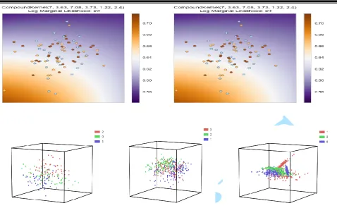
Figure 4.1. The classification of the multiclass high dimensional data
The charts above depicted the classification of the multiclass high dimensional data using Gaussian process of different kernels.
REFERENCES
[AS06] Amine B., Sofiane B. B. - Bayesian Learning using Gaussian for Gas Identification, IEEE Transactions on instrumentation and measurement vol. 55, No 36, 2006.
[Fon17] Fonnesbeck C. -Fitting Gaussian Process Models in Python,
https://blog.dominodatalab.com/fitting-gaussian-process-models-python/, 2017.
[KPX00] Kaiguang Z., Popescu S., Xuesong Z. - Bayesian learing with Gaussian process for supervised classification of Hyperspectral Data, American Society for Photogrammetry and Remote Sensing, vol. 74, No. 10 pp. 1223-1234, 2000. [K+13] Kemmler M., Rodner E., Wacker E.
S., Denzler J. - One-class classification with Gaussian Process, Pattern recognition 46 (3507-3518) www.elsevier.com/locale/pr, 2013.
[Olo17] Oloyede I. - Bootstrapping Supervised
Classifier Paradigm Annals. Computer
Science Series. 15th Tome 2nd Fasc.,
160-167, 2017.
[Rad98] Radford M. N. - Regression and classification using Gaussian process priors, Bayesian statistics 6, J.M. Bernardo, J.O. Berger, A.P. Dawid and A.F.M. Smith (EDs.), 1998.
[RW06] Rasmussen C. E., William C. K. - Gaussian Process for machine learning, The MIT press pp 33-52 www.gaussianprocess.org/gpml, 2006.
[SMT03] Shi J. Q., Murray-Smith R.,
Titterington D. M. - Bayesian
regression and classification using
mixtures of Gaussian processes, Int. J.
Adapt. Control Signal Process.; 17:149–
161 (DOI: 10.1002/acs.744), 2003.
[WR96] Williams C. K. I., Rasmussen C. E. - Gaussian Process for Regression, in D.S. Touretsky, M.C.Mozer and M.E. Hasselmo (Eds.): Advances in Neural Information Processing Systems 8, pp 514-520. MIT press, 1996.
[YSC11] Yi G., Shi J.Q., Choi T. - Penalized
Gaussian Process Regression and Classification for High-Dimensional
Nonlinear Data. Biometrics 67, 1285–
1294. DOI: