www.wind-energ-sci.net/1/237/2016/ doi:10.5194/wes-1-237-2016
© Author(s) 2016. CC Attribution 3.0 License.
Effect of Reynolds number and inflow parameters on
mean and turbulent flow over complex topography
Ryan Kilpatrick1,3, Horia Hangan1,2, Kamran Siddiqui1,3, Dan Parvu1,2, Julia Lange4, Jakob Mann4, and Jacob Berg4
1WindEEE Research Institute, University of Western Ontario, London, Ontario, N6M 0E2, Canada 2Department of Civil and Environmental Engineering, University of Western Ontario, London,
Ontario, N6A 5B9, Canada
3Department of Mechanical and Materials Engineering, University of Western Ontario, London,
Ontario, N6A 5B9, Canada
4DTU Wind Energy, Technical University of Denmark, Frederiksborgvej 399, 4000 Roskilde, Denmark
Correspondence to:Ryan Kilpatrick ([email protected])
Received: 9 May 2016 – Published in Wind Energ. Sci. Discuss.: 23 May 2016 Revised: 27 September 2016 – Accepted: 11 October 2016 – Published: 17 November 2016
Abstract. A characterization of mean and turbulent flow behaviour over complex topography was conducted using a large-scale (1:25) model in the WindEEE Dome at Western University. The specific topographic feature considered was the Bolund Hill escarpment facing westerly winds. A total of eight unique inflow conditions were tested in order to isolate the impact of key parameters such as Reynolds number, inflow shear profile, and effective roughness, on flow behaviour over the escarpment.
The results show that the mean flow behaviour was generally not affected by the Reynolds number; however, a slight increase in speed-up over the escarpment was observed for cases with lower inflow roughness. The shape of the inflow wind shear profile also had a minor impact on the mean flow near the escarpment. More significant effects were observed in the turbulent flow behaviour, where the turbulent kinetic energy (TKE) over the escarpment was found be a strong function of inflow roughness and a weak function of the Reynolds number. The local change in the inflow wind shear was found to have the most significant influence on the TKE magnitude, which more closely approximated the full-scale TKE data, a result which had not been previously observed in wind tunnel modelling of this topography.
1 Introduction
Wind turbines over the last few decades have emerged as a reliable and cost-competitive means of producing clean, renewable electricity. Although typically built on relatively flat terrain such as plains and farmland, wind farms are in-creasingly being placed in more rugged, or complex, terrain, marked by abrupt changes in elevation (Palma et al., 2008).
These sites often have strong wind resources, yet design-ing wind farms for these regions involves additional chal-lenges due to the changes imposed by the terrain on the three-dimensional structure of the wind, such as speed-up regions, changes to the wind shear profile, large vertical wind
and Hangan, 2013) compared to field measurements and are making inroads with industry, although they come with the trade-off of higher computational cost (Ayotte, 2008; Ay-otte et al., 2010). These advanced models generally require a higher degree of user input and experience, and thus results can be significantly affected by changes to boundary con-ditions, turbulence closure models, and other parameters, as shown for example in the wide spread of computational fluid dynamics (CFD) results in the Bolund blind comparison ex-ercise (Bechmann et al., 2011).
Thus, a better understanding of the wind regime in com-plex terrain, from a fundamental fluid dynamics perspective, is critical, given the opportunities for improved overall wind turbine performance including higher annual electricity pro-duction and reduced fatigue loading and associated mainte-nance costs (Peinke et al., 2004; Berg et al., 2011). This im-proved understanding of the flow behaviour can be used by modellers to select appropriate boundary conditions and tur-bulence models with greater confidence. One area that is not fully understood, and forms the subject of this study, is the sensitivity of the mean and turbulent response of the flow over complex topography to changes in the inflow condi-tions.
1.1 Wind tunnel modelling of flow over topography In order to improve computational models, the model results need to be validated against actual flow conditions. Full-scale testing is ideal for this purpose; however, due to the lack of control of inflow conditions and the significant testing cost, time, and effort required, wind tunnel modelling has served as a valuable tool for development and validation of both nu-merical and analytical models (Ayotte and Hughes, 2004). Provided that certain conditions are met, measurements taken of the flow across a scale model can provide very useful and repeatable representations of full-scale conditions as well as benchmarking for the validation of numerical and analytical models. The controlled environment of the wind tunnel pro-vides a means of isolating the effects of various parameters on the mean and turbulent flow behaviour, which is usually not possible in the field.
There are several examples of wind tunnel experiments conducted on flow over scale models of real topography for the purpose of wind resource assessment and wind turbine siting. These include isolated hill cases such as Askervein Hill (Taylor and Teunissen, 1987), Kettles Hill (Salmon et al., 1988), and more recently Bolund Hill (Berg et al., 2011), as well as highly topographically complex regions with mul-tiple hills and valleys (Chock and Cochran, 2005; Rasouli et al., 2009; McAuliffe and Larose, 2012).
1.2 Bolund experiment
The Bolund experiment arose from the need for additional model validation of flow over complex terrain, extending the
Askervein Hill Project of the early 1980s by offering steeper terrain and thus a greater challenge for numerical models to resolve. Bolund Hill is a peninsula located near Roskilde, Denmark, and is characterized by a long upwind open fjord fetch, a steep escarpment, and a long flat section on top of the island. The Bolund topography is geometrically similar to a typical wind turbine site in complex terrain, albeit on a smaller scale, and is suited as a test site given its well-defined, undisturbed inflow conditions, neutral atmospheric stratification, and relative absence of thermal and Coriolis effects (Berg et al., 2011). Although Bolund is a small hill, approximately 12 m high by 75 m wide and 130 m long, sim-ilarity laws allow for upscaling by 10–30 times under neutral atmospheric stratification.
Studies of the wind flow over Bolund Hill include the original field campaign (Berg et al., 2011), follow-up lidar measurements of the escarpment wake (Lange et al., 2016a), computational and physical modelling of the hill as a part of the blind comparison test (Bechmann et al., 2011), wind tun-nel modelling (Yeow et al., 2015), LES modelling (Diebold et al., 2013), and wind tunnel and LES modelling (Conan et al., 2016). During the field campaign, measurements were taken via 35 anemometers on 10 masts, positioned along two main incoming flow directions referred to as line A (239◦) and line B (270◦). These were the benchmark measurements against which the results of subsequent modelling efforts have been compared. A detailed diagram of the Bolund to-pography, with mast positions and flow directions, appears in Berg et al. (2011).
1.3 Present study: characterization of mean and turbulent flow over Bolund across a range of input conditions
2 Experimental setup
The experimental setup, comprising the wind tunnel facil-ity, the topographic model, instrumentation, and measure-ment procedure is described in the sections below for both the WindEEE and BLWTL experiments.
2.1 WindEEE facility
The WindEEE dome is a unique wind research facility de-signed to simulate a wide variety of wind flow patterns in-cluding rotational (axisymmetric) and boundary layer flows on larger laboratory scales than conventional wind tunnels. A general description of the facility is provided in Hangan (2014). The hexagonal test chamber, with diagonal length of 25 m, is enclosed in a return air chamber of 40 m diagonal length. The WindEEE test chamber contains 106 fans, whose wind speed and direction can be varied independently to pro-duce the desired flow conditions. The facility can be operated in two distinct modes: multi-fan wind tunnel or axisymmetric mode. The present experiments were conducted exclusively under the former configuration, with only the fans along one wall of the hexagon in operation. The fans are mounted in an array format, i.e. four rows of 15 fans each, for a total of 60 fans. Each of these fans are 0.8 m in diameter and oper-ate at approximoper-ately 25 m s−1at a nominal power of 30 kW. Each fan is equipped with variable speed drive and can be in-dividually controlled to create a customized flow pattern. A contraction section was positioned immediately downwind of the 60-fan wall to improve flow uniformity and increase flow speed across the 5 m diameter test section (turntable) in the centre of the chamber. A trip and a series of spires were employed downwind of the fan wall, within the contraction section, to enhance turbulence intensity.
In addition to individual fan control, the WindEEE facil-ity also provides the abilfacil-ity to set roughness element position and height, allowing physical simulation of a wide range of incoming atmospheric boundary layer (ABL) flow profiles. There are over 1500 roughness elements in the test cham-ber, each with a maximum height of 30 cm. The present ex-periment employed only the roughness element sections in the vicinity of the contraction, upwind of the turntable. Two different roughness element configurations, both with a uni-form element height of roughly 7.5 cm, were used for the WindEEE experiment, hereinafter referred to as RC1 and RC2. For RC1, all of the roughness elements upwind of the turntable were raised, whereas for RC2, one block of about 80 elements immediately upwind of the turntable was low-ered to the floor, resulting in a lower effective roughness value than that of RC1.
2.2 Bolund scale model
The 1:25 scale model of Bolund Hill was produced by com-puter numeric control (CNC) milling of several large blocks
Figure 1.Schematic of WindEEE experimental setup.
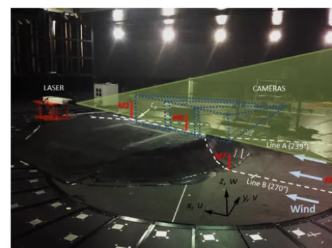
Figure 2.Photograph of the WindEEE experimental setup.
of expanded polystyrene (EPS) according to topographical data of the island. These blocks were then glued together and painted black with latex paint. The overall size of the model was roughly 4.5 m across, 0.5 m high, and 3.5 m long. A solid ramp with slope of roughly 45◦was constructed from EPS and fastened to the downwind edge of the model to provide a smooth transition and reduce unwanted flow separation. The model was positioned in the chamber such that the escarp-ment edge was roughly 12.4 m from the 60-fan wall, and the plane of measurement (along line B) was parallel to the flow direction. A simplified schematic diagram of the WindEEE experimental setup is shown in Fig. 1, while a photograph of the experimental setup is presented in Fig. 2. The centre point of the model,Cp, was set as the reference location (X=0),
which was also the intersection of lines A and B, as per the full-scale co-ordinate system (see Fig. 2).
2.3 PIV measurement
PIV was used to measure the two-dimensional velocity field in a vertical plane above the model, along line B, in the vicin-ity of the escarpment. The measurement region encompassed a rectangular area extending roughly from Z=11.4 m to
abso-lute height above sea level, while lowercasezdenotes height measured from the hill surface. Three 12 megapixel cameras (IO Industries Flare 12M125-CL), each with 105 mm f/2D Nikon AF DC-NIKKOR lenses, were used to capture images. The cameras were positioned in a row parallel to the flow di-rection, facing the model at a distance of roughly 3.55 m from the camera lens to the measurement plane, at a height such that the bottom of the camera frame of view was just below the hill surface. Camera resolution was 4096×3072 pixels, and the corresponding measurement field of view for each camera in the current setup was about 0.78 m wide by 0.58 m high. The horizontal positions of the cameras were selected such that the overlap between the adjacent fields of view was at least 10 %, ensuring spatial continuity of flow measure-ments. The overlap between cameras 1 and 2 was 0.167 m and 0.088 m between cameras 2 and 3, with camera 1 being the most upwind. Thus the combined measurement area was roughly 2.09 m wide by 0.58 m high (52.3 m×14.5 m in full-scale co-ordinates).
A Litron Nano Piv Series dual-cavity Nd:YAG laser with an energy of 425 mJ pulse−1, a wavelength of 532 nm, and a beam diameter of 9.5 mm was used to illuminate the flow field. The laser was positioned directly behind the model, pointing upwind, coincident with line B, with the laser head roughly 0.60 m off the ground, as shown in Fig. 2. A 50◦ cylindrical lens was positioned immediately in front of the laser head to convert the beam into a two-dimensional sheet. The laser was synchronized to the cameras and the frame grabber. In this study, the pulse repetition rate for each laser cavity was set at 9 Hz resulting in an image acquisition rate of 18 frames per second for each camera or 9 Hz for each image pair. The images were acquired via IO Industries Coreview software as 8 bit grayscale images in Tagged Image File For-mat (TIFF) forFor-mat. PIV data were recorded for 5 m per test case, providing roughly 2700 image pairs. An Ultratec CLF-4460 commercial fog generator, positioned in the dome’s up-per plenum, was used to seed the test chamber with non-toxic, water-based smoke that served as the tracer. Seeding particle size is estimated to be∼5 µm based on the estima-tion by Ayotte and Hughes (2004) for a commercial fog gen-erator similar to the one used in the present study.
2.4 Cobra probe measurement
Cobra probes, manufactured by Turbulent Flow Instrumen-tation Pty Ltd., are dynamic multi-hole pressure probes for measuring all three components of mean and fluctuating ve-locities and static pressure. In the present experiment, Cobra probe measurements were taken at an upwind reference lo-cation, as well as at a few positions along the hill. A vertical array of eight Cobra probes was used, with spacing between probes ranging from roughly 5 cm near the bottom of the ar-ray to 15 cm near the top. The total vertical measurement distance was about 60 cm, or 15 m in full-scale co-ordinates. The upwind reference position was located 4.44 m upwind
Figure 3.Photograph of the BLWTL experimental setup.
ofCpin the model scale (2.25 m upwind of the escarpment
leading edge), orX= −111 m in the full scale. Although it was initially intended for the Cobra probe position to coin-cide with the full-scale upwind reference mast M0, located atX= −180.8 m, this was not possible in the current setup due to the proximity of the model to the contraction open-ing. However, the selected location was deemed to be suf-ficient as a reference location given that it was far enough from the fan wall to assume fully mixed flow and far enough from the model to avoid significant slow-down effects. Along the hill, Cobra probe measurements were taken at the es-carpment edge (X= −54.7 m), at M6 (X= −46.1 m), and at M3 (X=3.2 m), where values in parenthesis are full-scale co-ordinates. Due to time constraints, Cobra probe measure-ments at these positions were not taken for each of the PIV test case configurations. The probe array was mounted either on a stationary floor rack or fixed to the overhead rail sys-tem and moved to various positions along line B. All Cobra probe measurements were conducted at an acquisition rate of 10 000 Hz, an output to file rate of 1250 Hz, and a sampling time of 120 s.
2.5 BLWTL experimental setup
upwind end of the tunnel; however, no active roughness ele-ments were used in order to simulate inflow conditions with an ABL profile over a smooth surface. The measurements were conducted at a wind speed of 4.6 m s−1, which corre-sponds to a Reynolds number of approximately 3.6×10⁴, us-ing the maximum height of the hill (0.117 m in model scale) as the characteristic length.
Cobra probe measurements were conducted along vertical profiles at model-scale positions equivalent to the full-scale co-ordinates of M0, M7, M6, M3, and M8, as well as at the escarpment (X= −54.7 m in full scale). The vertical velocity profile was obtained by using two Cobra probes mounted to the wind tunnel traverse system, and the vertical position was incremented after each sample by 12.7 mm in model scale (1.27 m in full scale) near the floor and 50–100 mm (5–10 m full scale) higher up. The vertical extent of the measurements was about 1.2 m from the floor (equivalent to 120 m in full scale). PIV measurements were conducted as well but are not presented here due to a number of issues with data quality.
3 Data processing
The methods of data processing, for both PIV and Cobra probe measurements, are described in the following sections.
3.1 PIV data processing
PIV instantaneous velocity fields were obtained by cross-correlating the interrogation regions in the first image of the image pair with the corresponding search regions in the sec-ond image. An in-house algorithm implemented in image processing software Heurisko®developed by AEON Verlag & Studio GmbH & Co. KG was used for the PIV data pro-cessing. The search window and interrogation window sizes were set as 128 and 64 pixels, respectively, while the grid distance was 16 pixels, with 75 % overlap for the interroga-tion windows. This resulted in a nominal spatial resoluinterroga-tion of roughly 3.04 mm for the velocity fields. Spurious vectors were identified and corrected using a local median test de-veloped by Siddiqui et al. (2001). Subsequently, mean fields were calculated by averaging the respective velocity compo-nent (streamwise,U, and vertical,W, in the present case) at each grid point over the sampling time. The turbulent veloc-ity fields were computed by subtracting the mean velocveloc-ity from the instantaneous velocity at each grid point in a given velocity field. These two steps were performed using an in-house code in MATLAB.
PIV statistics were calculated in a manner analogous to Yeow et al. (2015) to enable direct comparison. Mean flow speed,S, was calculated using the two mean wind compo-nentsUandWfrom the PIV measurement plane (see Fig. 2) as follows:
S=U2+W2
1/2
. (1)
Results shown throughout this work are often expressed as a normalized speed-up ratioS(x, z)/S0(z), whereS0(z) is the
inflow reference speed at the same height. Since the inflow Cobra probe measurements were taken only up to a height of 0.68 m above the floor and the PIV windows reached a height of about 1 m, extrapolation was carried out according to the following logarithmic law (Manwell et al., 2009):
U(z)/U(zr)=ln
z z0 /ln z r z0 , (2)
wherezris the reference height. While ideally the inflow
pro-file would have been measured up to the maximum height of the PIV measurement window, this was not feasible with the equipment available at the time of the experiments. Thus, given these limitations, the logarithmic law was selected as the best fit to the measured data. Mean turbulent kinetic en-ergy (TKE),k, was calculated according to
k=
u02+w02/2, (3)
whereu0 and w0 represent the fluctuating velocity vectors. The TKE increment1kwas obtained by subtracting the in-flow reference TKEk05 at a fixed height ofZ=5 m in full
scale (0.2 m in model scale) from the measured TKE at each PIV grid position and normalizing by the square of the inflow reference speed, again consistent with Yeow et al. (2015):
1k=hk(x, z)−k05
i
/S02(z). (4)
Despite efforts to properly align the three cameras, some minor discrepancies were observed in the velocity data recorded by each camera. For mean wind speeds, error be-tween camera frames typically ranged from about 2–4 %, with slightly more error in the highly turbulent region close to the escarpment and just above the model surface. To im-prove the clarity of presentation, a frame stitching algorithm was implemented to smooth the data within the overlap re-gion between camera frames. At each point in the overlap-ping region, a weighted average of the data at the two over-lapping nodes was taken, such that data points closer to one camera or another were weighted more heavily towards that camera’s values. The weightings varied linearly from 0.5 for each camera at the centre of the overlap region (equal weight-ing) to 1 and 0 on one side and 0 and 1 on the other.
3.2 Cobra probe data processing
the PIV results, which is analogous to the approach adopted by Yeow et al. (2015) for hot-wire measurements. However, when comparing the WindEEE and BLWTL inflow profiles, measured with Cobra probes, against the full-scale data from upwind reference mast M0, all three wind speed components from the Cobra probe data were used.
4 Inflow profiles
Inflow conditions for the various test cases, for both the WindEEE and BLWTL experiments, are described in the sec-tions below.
4.1 WindEEE fan configuration
For the present set of experiments, the 60 fans were operated using four different configurations, which were selected in an attempt to match the full-scale incoming wind profile, as well as to produce a range of Reynolds numbers (see Table 1):
a. all fans running at 20 % of the maximum fan rpm
b. all fans running at 30 % of the maximum fan rpm
c. all fans running at 50 % of the maximum fan rpm
d. fans in row 1, 2, and 4 running at 50 % and fans in row 3 at 75 % of the maximum fan rpm; for reference, fan row 1 is at floor level.
The notation for each test case was set based on the inflow wind speed and the inflow surface roughness. That is, each of the four fan configurations are identified by the mean stream-wise incoming wind speed at the model escarpment height in metres per second (i.e. U5, U8, U14, U15) and one of two roughness configurations (RC1 or RC2), where RC1 corre-sponds to higher roughness. For example, case U5RC1 cor-responds to the test case conducted at the inflow condition of 5 m s−1wind flowing over higher roughness. These
combi-nations yielded eight unique flow configurations representing the WindEEE PIV test cases described throughout this work, as listed in Table 1.
4.2 WindEEE inflow parameters
Cobra probe measurements taken at the upwind reference po-sition were used to determine inflow conditions, with mean speed, TKE, Reynolds shear stress, and integral length scales being of primary interest for the present study. Upwind mean speedS0and TKEk0are shown in Fig. 4 along with the
full-scale measurements at M0 (Berg et al., 2011). Inflow profiles of Reynolds shear stress and integral length scales are shown in Fig. 5. The Reynolds number was calculated according to
Re=Uhh
ν , (5)
where the characteristic length h is the hill height, Uh is
the inflow streamwise velocity ath, and ν is the kinematic viscosity of air. The Reynolds numbers in Table 1 use the model hill height h=0.468 m. For the test cases with the same fan configuration but different roughness configuration, the Reynolds number was almost identical. Inflow turbulence intensity at hill height Iuh0 was approximately 0.13 for all WindEEE test cases. The boundary layer heightδwas taken as the height at which the mean streamwise velocity was equal to 0.99U∞, whereU∞is the free-stream velocity. The ratio of boundary layer height to hill heightδ/ hranged from 3.3 to 3.6 for the WindEEE cases.
For the present study, which focuses mainly on how in-flow conditions affect in-flow behaviour over the escarpment, the means by which the inflow parameters are calculated are important, as there is often some variability depending on the method of calculation. For example, friction velocityu∗can be determined using several different methods, which often show considerable differences between them (Weber, 1999). To compare the variability of the resulting normalized inflow profiles for the WindEEE experiment, the friction velocity was calculated using four different methods. For Method 1, friction velocity was calculated according to Eq. (6), as per Weber (1999), using only the longitudinal component of the Reynolds stress vector. This is analogous to the method used by Berg et al. (2011) to calculate friction velocity using data from the inflow reference mast M0 at a height of 5 m above sea level in the Bolund field campaign.
u∗=
−u0w01/2 (6)
Method 2 adds the spanwise Reynolds stress component (Ly, 1993; Weber, 1999) and always produces a higher value ofu∗ than Method 1. It is similar to the method used in Bechmann et al. (2011) and is given by
u∗=
u0w02+v0w02 1/4
. (7)
For Methods 1 and 2, a single reference valueu∗05was taken as the friction velocity at a reference height ofZ=5 m in full scale (0.2 m in model scale), consistent with the approach used by Bechmann et al. (2011) and Yeow et al. (2015). In an undisturbed boundary layer profile, the region of con-stant Reynolds shear stress has been shown to correspond to the equilibrium sub-layer where TKE production balances with the dissipation (Tritton, 1977). For the WindEEE exper-iments, the three data points closest to the floor for each test case were found to be within this constant shear stress region (see Fig. 5a). The reference height used for Methods 1 and 2,
Figure 4.WindEEE inflow profiles of(a)mean flow speed and(b)TKE, normalized by friction velocity obtained using Method 1.Sandk
calculated using all three components of wind speed from Cobra probe measurements.Zco-ordinates shown in full-scale units.
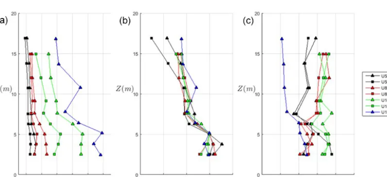
Figure 5. WindEEE inflow profiles: (a)Reynolds shear stress magnitudes, (b) Reynolds shear stress normalized by friction velocity (Method 1), and(c)integral length scales of the streamwise velocity component, normalized by hill heighth.
isκ/u∗and theyintercept is ln (z0) (Manwell et al., 2009):
ln (z)=
κ u∗
U(z)+ln (z0), (8)
wherezis the vertical height above the ground,U(z) is the streamwise wind speed at that height, and the von Karman constant κ was considered to be 0.41. The line of best fit was drawn only through data points residing within the re-gion of constant shear stress. Method 4 follows the approach of Akomah et al. (2011), whereu∗is considered to be equal to the average of the values of u∗ values at heights within the region of constant shear stress. The values of u∗
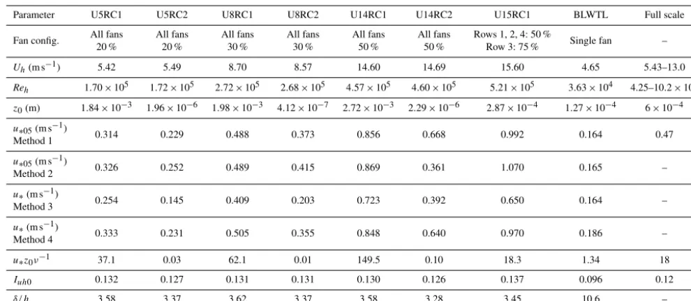
esti-mated using each of the four methods are presented in Ta-ble 1. As the data show, the difference between the highest and lowest estimate was relatively high, ranging from about 15 to 50 % depending on the test case. Thez0values shown
in Table 1 were obtained using Method 3 and are presented in full-scale units. The values show a clear distinction between the RC1 cases (z0∼10−3m) and RC2 cases (z0∼10−6m).
The RC1 cases fell within the fully aerodynamically rough regime, where friction Reynolds numberu∗z0ν−11 (see
Table 1.Inflow parameters for WindEEE and BLWTL test cases.
Parameter U5RC1 U5RC2 U8RC1 U8RC2 U14RC1 U14RC2 U15RC1 BLWTL Full scale
Fan config. All fans All fans All fans All fans All fans All fans Rows 1, 2, 4: 50 % Single fan – 20 % 20 % 30 % 30 % 50 % 50 % Row 3: 75 %
Uh(m s−1) 5.42 5.49 8.70 8.57 14.60 14.69 15.60 4.65 5.43–13.0
Reh 1.70×10⁵ 1.72×10⁵ 2.72×10⁵ 2.68×10⁵ 4.57×10⁵ 4.60×10⁵ 5.21×10⁵ 3.63×10⁴ 4.25–10.2×10⁶
z0(m) 1.84×10⁻³ 1.96×10⁻⁶ 1.98×10⁻³ 4.12×10⁻⁷ 2.72×10⁻³ 2.29×10⁻⁶ 2.87×10⁻⁴ 1.27×10⁻⁴ 6×10−4
u∗05(m s−1) 0.314 0.229 0.488 0.373 0.856 0.668 0.992 0.164 0.47
Method 1
u∗05(m s−1) 0.326 0.252 0.489 0.415 0.869 0.361 1.070 0.165 –
Method 2
u∗(m s−1)
0.254 0.145 0.409 0.203 0.723 0.392 0.650 0.164 – Method 3
u∗(m s−1)
0.333 0.231 0.505 0.355 0.848 0.640 0.970 0.186 – Method 4
u∗z0ν−1 37.1 0.03 62.1 0.01 149.5 0.10 18.3 1.34 18
Iuh0 0.132 0.127 0.131 0.131 0.130 0.126 0.137 0.096 0.12
δ/ h 3.58 3.37 3.62 3.37 3.58 3.28 3.45 10.6 –
Roughness lengths shown in full scale. The inflow profile for case U15RC2 was not measured due to an oversight, and as a result the U15RC2 PIV results were normalized against the U15RC1 inflow data.
u∗z0ν−1<0.2; therefore, a dependence ofz0 onu∗ is ex-pected. Values ofu∗z0ν−1for each test case are indicated in
Table 1. The full-scale roughness measured at mast M0 was
z0=3×10⁻⁴(Berg et al., 2011), so the U15RC1 case shows
the closest match among the WindEEE test cases.
4.3 Comparison between inflow profiles
When normalized byu∗05 (Method 1), a clear separation is observed between the profiles with higher roughness (RC1) and those with lower roughness (RC2), with the RC2 group having higher normalized mean wind speed as well as TKE (see Fig. 4). Comparison of the inflow mean speeds for the test cases with the full-scale data shows that all model-scale values are lower than the full-scale wind speeds, with the ex-ception of U5RC2, whereas the normalized TKE profiles are all higher than the full-scale profile, illustrating the inherent difficulty in matching both the mean wind speed and TKE profiles with the full-scale values. The shape of the TKE pro-files is in contrast to the wind tunnel experiment conducted by Yeow et al. (2015), whose normalized TKE inflow pro-files were lower than the full-scale values and decreased with height. Most of the WindEEE normalized TKE profiles are relatively vertical between z=5 m and z=12 m, which is consistent with the full-scale data, although having only two full-scale data points available from the reference mast M0 in the field campaign, none of which were above a height of 12 m (i.e. just above escarpment height), is a limiting factor in determining whether a good match to the full-scale condi-tions has been achieved. When normalized using Method 2 (not shown), profiles are similar to those shown for Method 1 but shifted slightly to the left, given the slightly higher
val-ues ofu∗. There is also less separation between the RC1 and RC2 groups. Inflow profiles determined using Method 3 pro-duce a better match to the full-scale data for mean speed for the RC1 group although they remain higher for TKE. For the RC2 group, profiles remain slightly higher than full scale for mean speed and are shifted even further to the right for TKE, due to the higher values ofu∗. Profiles normalized us-ing Method 4 are similar to those of Method 1, with pro-files collapsing to a greater extent within the RC1 and RC2 groups.
Upwind Reynolds shear stress −u0w0 as a function of height is shown in Fig. 5 for the WindEEE cases. Magnitudes of shear stress (Fig. 5a) are shown to increase with Reynolds number, and the higher roughness (RC1) cases exhibit con-sistently higher shear stress than the lower roughness (RC2) cases. When normalized byu2∗05, whereu∗is calculated us-ing Method 1 (Fig. 5b), the shear stress profiles generally tend to collapse, with some deviations, notably the lower values of the U5 cases at higher elevations and the higher value of the U15RC1 case near hill height (Z=11.73 m). The value of the non-dimensional Reynolds shear stress for U15RC1 is about 60 % higher than that of the U14RC1 case in this high shear region.
Inflow integral length scales in the streamwise direction
Luu are shown in Fig. 5c. Timescales were determined by
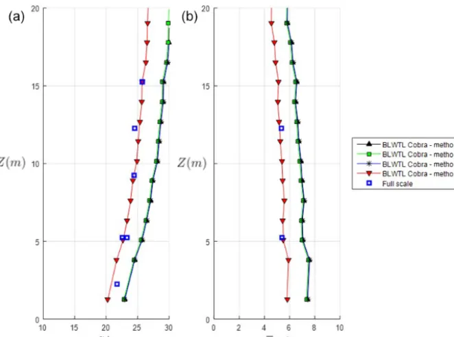
Figure 6.BLWTL inflow profiles of(a)mean flow speed and(b)TKE, normalized by friction velocity obtained using four different methods.
number. The difference is particularly large at hill height. Based on the results presented in Figs. 4 and 5, it can be inferred that the inflow profile for the shear case is character-ized by eddies with smaller average size and higher levels of momentum transport than for the uniform fan cases, particu-larly near hill height.
4.4 BLWTL inflow profiles
The key inflow parameters for the BLWTL Cobra probe mea-surements are shown in Table 1. Friction velocity was calcu-lated according to each of the four methods outlined above, and z0 was estimated using Method 3. Friction Reynolds
numberu∗z0ν−1was 1.39; thus, the inflow was in the
transi-tionally rough regime (Bowen, 2003). Figure 6 shows inflow profiles from the BLWTL Cobra probe data, measured at the inflow reference location ofX= −1.82 m in model scale (X= −182 m in full scale). Mean speed and TKE were nor-malized by friction velocity calculated using the four meth-ods identified above. The results show that the profiles for Methods 1–3 are quite close to each other and higher than the full-scale data points, while Method 4, with higher u∗, produced profiles shifted slightly to the left and matched par-ticularly well with the full-scale data. The reduction in nor-malized TKE with height was consistent with the inflow pro-files measured by Yeow et al. (2015) but different from the WindEEE and full-scale TKE profiles, which were relatively constant with height over the measurement region. Similar-ities between the inflow profile of the BLWTL experiment and those of Yeow et al. (2015) were expected given thatu∗
andz0are almost of the same order for both studies,
mak-ingu∗z0ν−1similar. Inflow turbulence intensity was roughly
0.1, andδ/ hwas 10.6 for the BLWTL case (see Table 1).
5 Results and discussion
The results are divided into two main sections: analysis of the mean flow behaviour, and analysis of the turbulent flow be-haviour. Most of the results presented were obtained from the WindEEE PIV data, while some additional data are presented from the WindEEE and BLWTL Cobra probe measurements.
5.1 Mean flow behaviour
con-Figure 7. Streamlines of mean velocity for various cases with roughness configuration RC1.
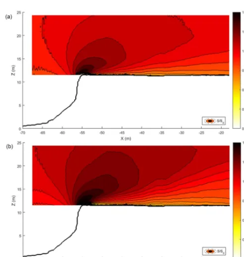
Figure 8.Contours of speed-up ratio (S/S0) for(a)U14RC1 and
(b)U15RC1.
clusion about the presence of a recirculation zone. An analy-sis of the probability of occurrence of negative instantaneous velocity vectors in the streamwise direction for each case was conducted in a manner analogous to Yeow et al. (2015). For all cases, it was observed that, apart from a very small near-surface region close to the escarpment leading edge, the probability of occurrence of negative vectors was less than 1 %, which further decreased with an increase in downwind distance and height. This is consistent with the results pre-sented by Yeow et al. (2015). The U15RC1 shear case had a relatively higher occurrence of negative vectors over a wider region above the hill surface compared to the uniform cases U14RC1 and U14RC2, which were similar to each other.
Contour plots of speed-up ratio for U14RC1 (Fig. 8a) and U15RC1 (Fig. 8b) clearly illustrate the speed-up region near the escarpment and the re-establishment of the bound-ary layer on top of the hill. The U5 and U8 contour plots (not shown) were very similar to the U14 case, analogous to the similarity observed in the streamline plots between the three cases. While speed-up is generally similar between the U14RC1 and U15RC1 cases, slightly higher values are ob-served for U15RC1 in the vicinity of the escarpment, and this case also shows a more elongated, oblong shape of the speed-up region at the escarpment edge. The Reynolds number for the two flows did not differ by a great amount (4.57×10⁵ for U14RC1 vs. 5.21×10⁵for U15RC1), i.e. much less than the difference in Reynolds number between the U5RC1 and U14RC1 cases, indicating that the difference in normalized mean flow behaviour can be most likely attributed to the higher inflow shear for the U15 case.
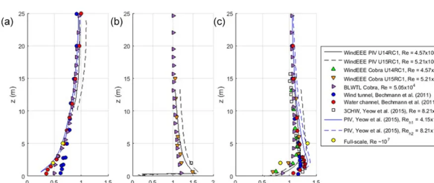
5.2 Mean flow comparison to previous experiments In addition to the full-scale measurements, results from pre-vious physical modelling of the Bolund Hill are available in the literature for comparison to the present results. These include wind tunnel and water channel experiments from the blind comparison (Bechmann et al., 2011), wind tunnel PIV and three-component hot-wire (3CHW) tests conducted by Yeow et al. (2015) on a 1:115 scale at two Reynolds numbers (4.15×10⁴and 8.21×10⁴), and wind tunnel PIV modelling conducted by Conan et al. (2016) on a 1:500 scale andRe=2.1×10⁴. Benchmarking the WindEEE Co-bra probe and PIV and the BLWTL CoCo-bra probe results from the present experiment against these data sets provides some validation of the present experimental procedure and also serves as an initial point of discussion on the differences be-tween conducting the same experiment on three scales, i.e. wind tunnel (Re∼104), WindEEE (Re∼105), and full scale (4.25×10⁶<Re<1.02×10⁷).
agree-Figure 9.Horizontal profiles of speed-up ratio from PIV and Cobra probe measurements (WindEEE and BLWTL cases) at(a)z=5 m and
(b)z=2 m above hill surface, with(c)showing hill profile. Results from full scale and other previous physical experiments presented for
comparison.
Figure 10.Vertical profiles of speed-up ratio for WindEEE and BLWTL cases at(a)M7 (X= −66.9 m),(b)escarpment (X= −54.7 m), and(c)M6 (X= −46.1 m). Results from full scale and other previous physical experiments presented for comparison.
ment is observed at position M7 upwind of the escarpment (Fig. 10a), with greater variability seen at the other two posi-tions (Fig. 10b, c), particularly atz <5 m.
5.3 Influence of inflow parameters on the mean flow The WindEEE experiments were conducted by changing one variable at a time, allowing for the influence of a particular modifier to the flow to be isolated and the resultant flow
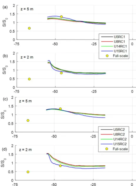
Figure 11.Horizontal profiles of speed-up ratio for(a)RC1 cases,
z=5 m, (b) RC1 cases, z=2 m, (c) RC2 cases, z=5 m, and
(d)RC2 cases,z=2 m.
5.3.1 Effect of Reynolds number and inflow wind profile on the mean flow
The horizontal profiles of the wind speed-up for four Reynolds numbers at full-scale heights ofz=5 m andz= 2 m above the island surface level are shown for two inflow roughness cases: higher roughness RC1 in Fig. 11a and lower roughness RC2 in Fig. 11b. Full-scale data are also plotted for reference. The normalized mean flow results show al-most identical trends for the three uniform fan speed cases (U5, U8, and U14) for both RC1 and RC2. This indicates an absence of Reynolds number effects on the mean flow over a Reynolds number range of 1.7×10⁵to 4.6×10⁵. The U15 case, however, with a modified inflow shear profile, displays different behaviour than the uniform fan speed cases. The U15RC1 peak speed-up is higher at the escarpment com-pared to the other RC1 cases (by about 9 % at z=5 m and by 7 % at z=2 m) and then changes to become relatively lower further downwind. For the U15RC2 case, speed-up is generally equal to or slightly lower than the other RC2 cases atz=5 m (Fig. 11c) and lower along horizontal locations at
z=2 m (Fig. 11d). In Fig. 12, a similar comparison is made along the vertical profiles at M6. Results show a trend
simi-Figure 12.Vertical profiles of speed-up ratio at M6 for(a)RC1
cases and(b)RC2 cases.
lar to that observed for the horizontal profiles, i.e. little differ-ence among the mean flow profiles in three uniform fan speed cases, with the RC2 profiles collapsing more closely. Again the U15RC1 case (Fig. 12a) shows different behaviour, with a higher speed-up than the other cases (i.e. about 9 % higher than U5RC1 atz=5 m) and also shows a better match to the full-scale data points. For RC2 (Fig. 12b), the U15 case gen-erally collapses with the others, with the only difference be-ing the relatively lower speed-up atz <4 m (i.e. 12 % lower than U5RC1 atz=2 m), which is again closer to the full-scale behaviour.
5.3.2 Effect of inflow roughness on the mean flow The comparison of speed-up profiles at the same Reynolds number but a different roughness configuration provides an insight into the effect of inflow surface roughness,z0, on the
RC1z0value being higher than the RC2 value by about 3
or-ders of magnitude. For the uniform fan speed cases, the peak speed-up atz=2 m was higher for the RC2 cases than RC1 by margins of about 6, 8, and 5 % for U5, U8, and U14, re-spectively. In the horizontal profiles, a lower inflow z0 was
found to generate a roughly 5 % higher peak speed-up at the escarpment, with a diminishing effect moving downwind. A different trend was observed for the U15 cases, where a slight reduction in peak speed-up of about 3 % was observed at the escarpment for the RC2 case, with the difference between the two roughness cases growing slightly moving downwind. At M6, the lower roughness cases showed a slightly better match to the full-scale data (see Fig. 12).
5.3.3 Effect of measurement and model resolution on the mean flow
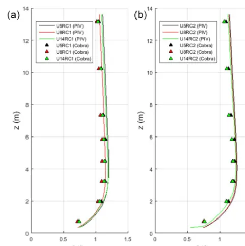
The Cobra probe measurements were taken under identi-cal fan speed and roughness element configurations to the PIV cases, although not simultaneously, and therefore from the mean flow perspective, they provide useful independent evidence for Reynolds number dependence. A comparison of speed-up ratio between PIV and Cobra probe measure-ments, for the three uniform fan speed cases, for both rough-ness configurations, along the same vertical profile at M6, is shown in Fig. 13. The results show very good matching between the two methods of measurements, with some sys-tematic bias error resulting in slightly lower speed-up for Cobra probe measurements, perhaps due to PIV calibration. Notwithstanding, very little evidence of Reynolds number dependence is observed between the Cobra probe profiles, confirming the trends observed earlier in the PIV data.
Now turning to the discussion on the effect of model res-olution on the mean flow, it is generally accepted by wind tunnel modellers that for bluff bodies submerged in deep boundary layers, Reynolds number effects are negligible for Re>(2–3)×104, particularly for flows without steady vor-tical regions (Lim et al., 2007). The BLWTL case and the WindEEE cases under uniform fan speed, as well as the two tests conducted by Yeow et al. (2015), atRe=4.15×10⁴and Re=8.21×10⁴, were all above this threshold. The WindEEE uniform fan speed cases are consistent with the literature in showing a lack of Reynolds number dependence. One would therefore expect to see Reynolds number independence pre-served between normalized speed-up profiles at the BLWTL scale (1:100) and the WindEEE scale (1:25), measured us-ing the same instrument, under similar inflow conditions. Such a comparison is made in Fig. 10, which shows speed-up profiles from Cobra probe measurements for the BLWTL and WindEEE cases. Some discrepancies are observed, particu-larly at M6 at z <5 m, where the WindEEE U14RC1 mea-surements were found to be higher than the BLWTL values by about 5 % and a better match to the full-scale measure-ments. It can therefore be concluded that the discrepancies between Cobra probe results observed at the two different
Figure 13.Vertical profiles of speed-up ratio from WindEEE PIV
and Cobra probe at M6 for(a)RC1 and(b)RC2.
model resolutions are unlikely to be due to Reynolds number effects but rather caused by other factors such as proximity of the measurement instrument to the surface, size of the in-strument relative to the model and surface roughness of the model.
5.4 Turbulent flow behaviour
The results for the turbulent flow are presented in a similar manner as for the mean flow behaviour in Sect. 5.1. To ob-tain a better insight into the overall turbulent flow behaviour, contour plots of the change in TKE1k over the same area as in the earlier speed-up plots are shown in Fig. 14a and b for U14RC1 and U15RC1, respectively. A highly turbulent region is observed at the escarpment, which dissipates mov-ing downwind. Several significant differences are observed between the two cases, with U15RC1 having a larger high-intensity TKE region near the escarpment and a longer and higher wake. The TKE increment also begins further upwind of the escarpment. The U5 and U8 TKE contour plots (not shown) were similar to the U14 case but with slightly lower values of1kthroughout.
5.5 Turbulent flow comparison with previous experiments
A comparison of horizontal profiles of WindEEE TKE in-crement against previous experimental results atz=5 m and
fea-Figure 14.Contours of mean TKE increment1kfor(a)U14RC1
and(b)U15RC1.
ture a shallow hump between M6 and M3 at z=5 m and a sharp spike between the escarpment and M6 at z=2 m. Both features are much more pronounced for the U15RC1 case compared to U14RC1. The Cobra probes were not able to capture the TKE spike to the same extent, also observed in the vertical profile at M6 (see Fig. 16). As was the case for the speed-up ratio, the U15RC1 case was observed to better approximate the full-scale values of1kthan the others.
5.6 Influence of inflow parameters on the turbulent flow Similar to the mean flow analysis, the effects of inflow Reynolds number, wind shear profile, upwind roughness, and model and measurement resolution on the turbulent flow be-haviour are discussed in the following sections.
5.6.1 Effect of Reynolds number and inflow wind profile on the turbulent flow
Figure 17 shows horizontal profiles of1kfor the four wind speed cases at RC1 and RC2, respectively. The two U15 pro-files stand out from the other cases – the peak TKE increment for U15RC1 was about 200 % higher than that for U14RC1 – and the discrepancy is much more significant than it was for the speed-up ratio. The TKE results indicate that changes in the flow behaviour above the escarpment can be attributed to changes in the inflow parameters and elicit the following question: which are the relevant non-dimensional parame-ters? As noted previously, the only difference between the
U14 and U15 cases was the 50 % increase in the operating speed of fans in the third row from the floor compared to all other fans. This induced a strong shearing effect at the in-terface between fan rows 2 and 3, about 2 m above the floor in model scale or 50 m in full scale, just over 4 times the hill height. The higher fan speed in the third row produced a slightly higher Reynolds number at hill height for the U15 cases than for the U14 cases, but the Reynolds number dif-ference was small compared to the difdif-ference between the uniform cases and thus unlikely to be a significant contrib-utor to the TKE difference. Similarly, the non-dimensional TKE profiles (see Fig. 4) show little difference between the U15RC1 case and the three other RC1 cases. As discussed, more significant differences between the shear and uniform cases were observed among the inflow profiles of Reynolds shear stress and integral length scale (see Fig. 5), parame-ters which are known to influence turbulence behaviour and momentum transport. As shown by the inflow profiles, by the time the flow reaches the upwind reference position, the shearing effect introduced at the fan wall for the U15 shear case appears to produce turbulence characterized by smaller eddies with higher momentum compared to the uni-form cases at the hill height. The results highlight the im-portant fact that a relatively small change to the inflow wind shear profile, even well above the height of the topography, can significantly affect the turbulent flow behaviour near the surface.
Among the three uniform fan speed horizontal profiles, there is little difference in TKE increment atz=5 m; how-ever, atz=2 m, peak TKE increment for the U14RC1 case is about 17 % higher than U5RC1 and 29 % higher than U8RC1 in the other two cases. A similar trend is observed for the RC2 cases, where peak TKE increment for U14RC2 is about 25 % higher than U5RC2 and 27 % higher than U8RC2, in-dicating a possible Reynolds number dependence in this re-gion. Vertical profiles of TKE increment at M6 were also plotted (see Fig. 18) for the RC1 and RC2 cases. The profiles for the uniform fan speed cases again tended to collapse, with the exception of the U14 cases below z=2 m. Peak TKE increment at M6 for U14RC1 was about 7 % higher than U5RC1, and 13 % higher than U8RC1 and the peak value for U14RC2 was about higher 10 % higher than U5RC2 and 14 % higher than U8RC2.
5.6.2 Effect of inflow roughness on the turbulent flow The influence of inflow roughness can be seen in Fig. 18. For the uniform fan speed cases, configuration RC2, with lower
z0, appeared to cause a moderate increase in peak TKE
Figure 15.Horizontal profiles of TKE increment1kfrom PIV and Cobra probe measurements (WindEEE and BLWTL cases) at(a)z=5 m and(b)z=2 m above hill surface, with(c)showing hill profile. Results from full scale and other previous physical experiments shown for comparison.
Figure 16.Vertical profiles of TKE increment1kfrom PIV and Cobra probe measurements (WindEEE and BLWTL cases) at(a)M7 (X= −66.9 m),(b)escarpment (X= −54.7 m), and(c)M6 (X= −46.1 m). Results from full scale and other previous physical experiments shown for comparison.
at different roughness configurations was about 13, 28, and 27 % for U5, U8, and U14, respectively, with the RC2 value being higher in each case. A negligible difference in TKE in-crement was generally observed between the two U15 cases at most locations. Peak TKE increment atz=5 m was about 7 % higher for U15RC1 than U15RC2. Thus, a change in the inflow roughness was observed to have a moderate effect on the TKE increment for the uniform fan speed cases, while the shear case appeared to be more resilient to changes in the inflow roughness.
5.6.3 Effect of model and measurement resolution on the turbulent flow
Figure 17.Horizontal profiles of TKE increment1kfor(a)RC1
cases atz=5 m,(b)RC1 cases atz=2 m,(c)RC2 cases atz=
5 m, and(d)RC2 cases atz=2 m.
capture the spike in TKE to the same extent as the PIV mea-surements, which may be partially due to the reverse flow at this location. Although Reynolds number effects may con-tribute to the higher TKE for the U14 PIV profile atz <3 m, Reynolds number independence appears to be almost com-pletely preserved among the three Cobra probe profiles all the way down to the hill surface. This observation once again raises the question of why the measurements using the 1:25 scale model at WindEEE are higher than those using the 1:100 BLWTL model and why they more closely approx-imate the full-scale measurements, as seen in Fig. 16c at M6. The resolution of the model and the ability to measure closer to the surface level thus appears to be one contributing factor. A separate study by Lange et al. (2016b) recently submitted for publication investigates the effect of sharpening the es-carpment edge. Preliminary analysis shows that this has a significant effect on the flow behaviour in the near-surface region.
6 Conclusions
An experimental investigation to characterize the mean and turbulent flow behaviour over a steep escarpment,
repre-Figure 18. Vertical profiles of TKE increment 1k at M6 for
(a)RC1 cases and(b)RC2 cases.
sented by the topography of Bolund Hill, was conducted on two distinct scales (1:100 and 1:25) by means of wind tun-nel testing using PIV and Cobra probes. A range of Reynolds numbers, boundary layer inflow profiles, and inflow rough-ness values were examined. At WindEEE, three uniform fan profiles and one modified shear profile were tested at two different inflow roughness configurations, for a total of eight unique sets of inflow conditions. These results, presented in the form of normalized speed-up and TKE increment, were compared to each other and to measurements from the field campaign and previous experimental work to attempt to es-tablish the relative contributions of the key inflow parameters to flow behaviour over the hill.
escarp-Figure 19.Vertical profiles of TKE increment1kfrom WindEEE
PIV and Cobra probe at M6 for(a)RC1 and(b)RC2 cases.
ment for the uniform fan speed cases, whereas for the shear case, lower roughness caused a slight reduction in speed-up, particularly near the surface. Slightly higher values of speed-up were observed for the 1:25 scale model compared to the 1:100 model, which are attributed to factors such as prox-imity of the instrument to the model surface or model surface roughness.
From the turbulent flow field data represented in the form of a TKE increment, a weak Reynolds number dependence was observed whereby TKE increased with an increase in the Reynolds number, but only in the highly turbulent shear layer near the escarpment. Lower inflow roughness also served to moderately increase peak TKE among the uniform fan speed cases. A much more significant TKE increase was observed for the shear profile case, where peak normalized TKE at a height of 2 m above the hill increased by over 200 % com-pared to the uniform fan speed case at a similar Reynolds number. Through modification of the inflow shear profile, the WindEEE facility was able to produce higher TKE in-crements, which were closer to full-scale measurements than those that had been achieved previously in conventional wind tunnels, indicating a promising trend for future work in char-acterizing flow over topography.
For the wind developer, these results reinforce the need for very careful and detailed assessment of wind turbine in-flow conditions in complex topography, as even very small changes to the inflow profile used in the modelling process can cause highly significant changes at turbine height, par-ticularly in the turbulent flow behaviour.
7 Data availability
The intention is to publish the data used in this paper for public use on a server in the near future. In the meantime, data can be obtained by contacting the authors.
Acknowledgements. The present work is supported by NSERC, CFI, and UWO, in addition to the Center for Computational Wind Turbine Aerodynamics and Atmospheric Turbulence funded by the Danish Council for Strategic Research, grant number 09-067216.
Edited by: J. Lundquist
Reviewed by: A. Cuerva and one anonymous referee
References
Akomah, A., Hangan, H., and Naughton, J.: Very high Reynolds number boundary layers over 3D sparse roughness and obstacles: the mean flow, Exp. Fluids, 51, 743–752, doi:10.1007/s00348-011-1086-2, 2011.
Ayotte, K. W.: Computational modelling for wind energy assessment, J. Wind Eng. Ind. Aerod., 96, 1571–1590, doi:10.1016/j.jweia.2008.02.002, 2008.
Ayotte, K. W. and Hughes, D. E.: Observations of boundary-layer wind-tunnel flow over isolated ridges of varying steep-ness and roughsteep-ness, Bound.-Lay. Meteorol., 112, 525–556, doi:10.1023/B:BOUN.0000030663.13477.51, 2004.
Ayotte, K. W., Sullivan, P. P., and Patton, E. G.: LES and wind tunnel modelling over hills varying steepness and roughness, Fifth International Symposium on Computational Wind Engi-neering (CWE2010), 23–27 May 2010, Chapel Hill, North Car-olina, USA, 2010.
Bechmann, A., Sørensen, N. N., Berg, J., Mann, J., and Réthoré, P.-E.: The Bolund experiment, part II: blind comparison of mi-croscale flow models, Bound.-Lay. Meteorol., 141, 245–271, doi:10.1007/s10546-011-9637-x, 2011.
Berg, J., Mann, J., Bechmann, A., Courtney, M. S., and Jørgen-son, H. E.: The Bolund experiment, Part I: Flow over a steep, three-dimensional hill, Bound.-Lay. Meteorol., 141, 219–243, doi:10.1007/s10546-011-9636-y, 2011.
Botta, G., Cavaliere, M., Viani, S., and Pospíšil, S.: Effects of hos-tile terrains on wind turbine performances and loads: The Acqua Spruzza experience, J. Wind Eng. Ind. Aerod., 74–76, 419–431, doi:10.1016/S0167-6105(98)00038-5, 1998.
Bowen, A. J.: Modelling of strong wind flows over complex terrain at small geometric scales, J. Wind Eng. Ind. Aerod., 91, 1859– 1871, doi:10.1016/j.jweia.2003.09.029, 2003.
Chock, G. and Cochran, L.: Modeling of wind speed ef-fects in Hawaii, J. Wind Eng. Ind. Aerod., 93, 623–638, doi:10.1016/j.jweia.2005.06.002, 2005.
Conan, B., Chaudhari, A., Aubrun, S., van Beeck, J., Hämäläinen, J., and Hellsten, A.: Experimental and numerical modelling of flow over complex terrain: the Bolund Hill, Bound.-Lay. Meteo-rol., 158, 183–208, doi:10.1007/s10546-015-0082-0, 2016. Diebold, M., Higgins, C., Fang, J., Bechmann, A., and
Hangan, H.: The Wind Engineering Energy and Environment (WindEEE) dome at Western University, Canada, Wind Engi-neers, JAWE, 39, 350–351, doi:10.5359/jawe.39.350, 2014. Lange, J., Mann J., Angelou, N., Berg, J., Sjoholm, M., and
Mikkelsen, T.: Variations of the wake height over the Bolund es-carpment measured by a scanning Lidar, Bound.-Lay. Meteorol., 159, 147–159, doi:10.1007/s10546-015-0107-8, 2016a. Lange, J., Mann, J., Berg, J., Parvu, D., Kilpatrick, R., Costache,
A., Chowdhury, J., Siddiqui, K., and Hangan, H.: For wind tur-bines in complex terrain, the devil is in the detail, Nature Energy, resubmitted, 2016b.
Lim, H. C., Castro, I. P., and Hoxey, R. P.: Bluff bodies in deep tur-bulent boundary layers: Reynolds-number issues, J. Fluid Mech., 571, 97–118, doi:10.1017/S0022112006003223, 2007.
Ly, L. N.: Effect of the angle between wind stress and wind ve-locity vectors on the aerodynamic drag coefficient at the air-sea interface, J. Phys. Oceanogr., 23, 159–163, doi:10.1175/1520-0485(1993)023<0159:EOTABW>2.0.CO;2, 1993.
Manwell, J. F., McGowan, J. G., and Rogers, A. L.: Wind energy explained, 2nd Edn., John Wiley & Sons Ltd., Chichester, West Sussex, UK, 2009.
McAuliffe, B. R. and Larose, G. L.: Reynolds-number and surface-modeling sensitivities for experimental simulation of flow over complex topography, J. Wind Eng. Ind. Aerod., 104–106, 603– 613, doi:10.1016/j.jweia.2012.03.016, 2012.
Palma, J. M. L. M., Castro, F. A., Ribeiro, L. F., Rodrigues, A. H., and Pinto, A. P.: Linear and nonlinear models in wind resource assessment and wind turbine micro-siting in complex terrain, J. Wind Eng. Ind. Aerod., 96, 2308–2326, doi:10.1016/j.jweia.2008.03.012, 2008.
Peinke, J., Barth, S., Böttcher, F., Heinemann, D., and Lange, B.: Turbulence, a challenging problem for wind energy, Physica A, 338, 187–193, doi:10.1016/j.physa.2004.02.040, 2004.
Rasouli, A., and Hangan, H.: Micro-scale CFD simulation for wind mapping over complex topographic terrains, J. Sol. Energ.-T. ASME, 135, 041005, doi:10.1115/1.4024124, 2013.
Rasouli, A., Hangan, H., and Siddiqui, K.: PIV measurements for complex topographic terrain, J. Wind Eng. Ind. Aerod., 97, 242– 254, doi:10.1016/j.jweia.2009.06.010, 2009.
Salmon, J. R., Teunissen, H. W., Mickle, R. E., and Taylor, P. A.: The Kettles Hill project: field observations, wind-tunnel simula-tions and numerical model predicsimula-tions for flow over a low hill, Bound.-Lay. Meteorol., 43, 309–343, doi:10.1007/BF00121711, 1988.
Siddiqui, K., Loewen, M. R., Richardson, C., Asher, W. E., and Jes-sup, A. T.: Simultaneous particle image velocimetry and infrared imagery of microscale breaking waves, Phys. Fluids, 13, 1891– 903, doi:10.1063/1.1375144, 2001.
Taylor, P. A. and Teunissen, H. W.: The Askervein Hill project: overview and background data, Bound.-Lay. Meteorol., 39, 15– 39, doi:10.1007/BF00121863, 1987.
Tritton, D. J.: Physical Fluid Dynamics, Van Nostrand Reinhold Co., New York 1977.
Walmsley, J. L. and Taylor, P. A.: Boundary-layer flow over topog-raphy: impacts of the Askervein study, Bound.-Lay. Meteorol., 78, 291–320, doi:10.1007/BF00120939, 1996.
Weber, R. O.: Remarks on the definition and estimation of friction velocity, Bound.-Lay. Meteorol., 93, 197–209, doi:10.1023/A:1002043826623, 1999.