U
NIVERSITA DEGLI`
S
TUDI DIT
RENTOINTERNATIONAL DOCTORATE SCHOOL IN INFORMATION AND COMMUNICATION
TECHNOLOGIES
XXIII CYCLE – 2012
Parametric Real-Time System Feasibility Analysis Using
Parametric Timed Automata
U
NIVERSITA DEGLI`
S
TUDI DIT
RENTOINTERNATIONAL DOCTORATE SCHOOL IN INFORMATION AND COMMUNICATION
TECHNOLOGIES
XXIII CICLO- 2012
Yusi Ramadian
Parametric Real-Time System Feasibility Analysis Using
Parametric Timed Automata
Luigi Palopoli (Advisor) Alessandro Cimatti (Co-Advisor) Thesis Committee
AUTHOR’S ADDRESS: Yusi Ramadian
Dipartimento di Ingineeria e Scienza dell’Informazione Universit`a degli Studi di Trento
via Sommarive 14, I-38050 Povo di Trento, Italy E-MAIL:[email protected]
Abstract
Real-time applications are playing an increasingly significant role in our life. The cost and risk involved in their design leads to the need for a correct and robust modelling of the system before its deployment. Many approaches have been proposed to verify the schedulability of real-time task system. A frequent limitation is that they force the task activation to restrictive patterns (e.g. periodic). Furthermore, the type of analysis carried out by the real-time scheduling theory relies on restrictive assumptions that could make the designers miss important optimization opportunities. On the other hand, the application of formal methods for verification of timed systems typically produces a yes/no answer that does not suggest any correction action or robustness margins of a given design.
This work proposes an approach to combine the benefits of formal method in terms of flexibility with the production of a clear feedback for the designers. The key idea is to use parametric timed automata to enable the definition of flexible task activation patterns. The Parametric Verification of Temporal Properties (PTVP) algorithm proposed in this work produces a region of feasible parameters for real-time system. All the parameter valuation within this region is guaranteed to make the system respect the desired temporal behaviour. In this way developers are provided with a richer information than the simple feasibility of a given design choice.
This method uses symbolic model checking technique to produce the result that is a union of poly-hedral regions in the parameter space associated with feasible parameters. It is implemented in the tool Quinq that is based on NuSMV3. The tool also implemented an optimization to speed up the search, such as using non-parametric model checker to find counterexamples (i.e. traces) related to the unfeasi-ble choices of parameters.
Two applications of the tool and of the underlying method to several real-time system examples are presented in this dissertation : periodic real-time system tasks with offset and heterogeneous distributed real-time systems. A work that applies the tool in collaboration with another real-time system analy-sis tool, Modular Performance Analyanaly-sis Toolbox, is also presented to show one of the many possible application of the method presented in this work.
In this work we also compare our approach to the state of the art in the field of sensitivity analysis of real-time systems. However, compared to the other tools and approaches in this field, the method offered in this work presents unique advantages in the generality of the system modelling approach and the possibility to analyse the entire region of feasibility of any desired parameter in the system.
Keywords
Formal method, real-time system, temporal verification, scheduling verification.
Acknowledgments
Bismillah hir Rahman nir Rahim, Alhamdulillah hi Rabbil Alameen, Praise be to Allah Almighty who al-ways provide me with everything more than I have ever asked to bring this PhD research and dissertation into completion.
For this PhD research I am deeply indebted to my supervisors, Luigi Palopoli and Alessandro Cimatti, who always have their faith in me and my thesis work and always been very supportive and helpful. They always provided me with fresh ideas of new directions and knowledge I needed for every obstacles I found throughout the research. I also appreciate all the moral supports they provided which play important role for me to conclude this work.
During the implementation I got significant supports by everyone in NuSMV developer team of Fondazione Bruno Kessler. Sergio Mover in particular has provided significant helps towards the hybrid extension of the work in the end. MathSAT developer, Alberto Griggio, has contributed his help through MathSAT tool since the beginning phase of this work up to the end with the additional existelim tool. I would also like to thank Alena Simalatsar and Roberto Passerone for the collaboration work we had.
All my love and forever gratitude to my beloved parents, Dra. Psi. Nurdiah Tedjowati and Farid Luthfi, M.M, who had given me never ending care, encouragement and support all the time that has enabled me to reach this point in my life. For my siblings, Reza Rahardian, Faddy Ardian, Denia Farah-dian. I would also like to thank very much my dearest husband, Tizar Rizano, for his support all along this PhD program. I could not be anything I am now without them.
Last, I hope that the work in this thesis will be of value and be my contribution for the knowledge in general.
Trento, April 24th 2012 Yusi Ramadian
Contents
Abstract i
Acknowledgements ii
1 Introduction 1
1.1 Problem Description . . . 1
1.2 Solution Overview . . . 2
1.3 Research Contribution . . . 2
1.4 Structure of the Thesis . . . 3
2 Real–time Design Challenges 4 2.1 Real–Time System . . . 4
2.1.1 Terminologies and Definitions . . . 7
2.2 Schedulability area problem formulation . . . 12
2.2.1 General Problem Formalization . . . 13
2.3 Example Scenarios . . . 14
2.4 Challenges . . . 18
3 Background Knowledge 20 3.1 Satisfiability Modulo Theory . . . 20
3.1.1 Logic Terms . . . 20
3.1.2 Satisfiability Modulo Theory . . . 21
3.1.3 Bounded Model Checking . . . 22
3.1.4 Tools . . . 23
3.2 Timed Automata . . . 24
3.2.1 Timed Automata Formal Notation . . . 24
3.2.2 Timed Automata Verification in NuSMV . . . 27
3.3 Formal verification for task scheduling feasibility . . . 32
3.3.1 The Task Activation Automata . . . 33
3.3.2 The Scheduler Automata . . . 33
3.3.3 NuSMV implementation of timed automata verification . . . 35
3.3.4 Sensitivity Analysis . . . 37
4 Real–Time System Sensitivity Analysis on Parametric Timed Automata 38 4.1 Parametric Timed Automata . . . 38
4.2 Modelling real–time system in PTA . . . 41
CONTENTS iv
4.3 Sensitivity analysis using PTA . . . 42
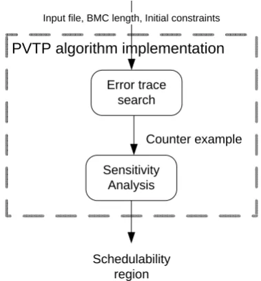
4.3.1 Parametric Verification of Temporal Properties (PTVP) algorithm . . . 42
4.3.2 Algorithm termination guarantee for periodic task sets . . . 44
4.4 Symbolic implementation . . . 46
5 Quinq Tool 49 5.1 Design of the tool - an overview . . . 49
5.1.1 General Architecture . . . 49
5.1.2 Components . . . 51
5.2 Specification Language . . . 53
5.2.1 SMV Language . . . 54
5.2.2 UPPAAL language . . . 54
5.2.3 High level modelling of periodic system . . . 55
5.2.4 Input language discussion . . . 56
5.3 PTVP Algorithm Implementation . . . 57
5.3.1 Error trace search . . . 58
5.3.2 Sensitivity analysis . . . 63
5.3.3 Iterative schedulability analysis for periodic tasks . . . 72
6 Application Examples 73 6.1 Standard Periodic Case . . . 73
6.1.1 Simple task set . . . 73
6.1.2 Large task set . . . 74
6.2 Arbitrary real–time system case . . . 75
6.2.1 System description . . . 75
6.2.2 System modelling . . . 77
6.2.3 Example result . . . 80
6.2.4 Example search optimization result . . . 83
6.2.5 Discussion . . . 83
7 MPA PTA 89 7.1 Motivation . . . 89
7.2 Real–Time Calculus . . . 90
7.3 System modelling . . . 91
7.3.1 From RTC-curves to event emitting PTA . . . 92
7.3.2 Generalized scheduler model . . . 94
7.4 Example case . . . 95
7.5 Discussion . . . 96
8 State of the Art 98 8.1 Schedulability analysis . . . 98
8.2 Sensitivity Analysis . . . 99
8.2.1 Analytical approach . . . 99
8.2.2 Sensitivity Analysis Tools . . . 100
8.2.3 Modeling and Analysis Suite for Real-Time Applications (MAST) . . . 100
CONTENTS v
8.2.5 Imitator . . . 102
9 Conclusion and Future Work 105 9.1 Conclusion . . . 105
9.2 Future Work . . . 106
A Quinq Usage 112 A.1 Sensitivity add-on . . . 112
A.1.1 Input . . . 112
A.1.2 Functions . . . 112
A.2 Periodic real–time system automatic schedulability analysis . . . 115
A.2.1 Input model . . . 115
A.2.2 Schedulability analysis for periodic case . . . 116
A.3 UPPAAL - NuSMV plugin . . . 117
A.3.1 UPPAAL model for template for NuSMV . . . 117
A.3.2 Schedulability analysis with optimized search . . . 118
A.4 Features . . . 119
List of Tables
5.1 Mapping between components and functionalities in Quinq . . . 54 6.1 The configuration of an example large periodic task system of 10 tasks with 5 parameters 76 6.2 Fixed parameter values in the two experiments . . . 80
List of Figures
2.1 The design process of correct design . . . 5
2.2 Figurative description of real-time job characteristic [31] . . . 8
2.3 The example of task with complex activation pattern . . . 9
2.4 The different states of a task . . . 12
2.5 The example of the feasibility regionR . . . 13
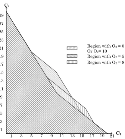
2.6 Feasibility regions of Scenario 1, Use case 1,in the domain ofC1 andC2 for different values ofO2 . . . 15
2.7 In the upper figure the system will fail usingO1 = O2 = 0, while in lower figure the system will succeed usingO1= 5andO2 = 1. . . 15
2.8 Regions of feasibility in the domain of O1 and O2 for Scenario 1, Use case 2. . . 16
2.9 Heterogeneous Communication System (HCS) . . . 17
2.10 Audio feasibility and error regions for∆ = 0,3,5,7. . . 18
2.11 Schedulability region of system . . . 19
3.1 A simple description on SMT solving schema . . . 22
3.2 T A1, an example of a task activation automata to be encoded in NuSMV. . . 24
3.3 A timed automata to be encoded in composition withT A1 . . . 26
3.4 An example of a periodic task activation automata . . . 33
3.5 The example of task activation and scheduler automata for 2 tasks . . . 36
4.1 Example of parametric timed automata: tasks activation . . . 39
4.2 Example of parametric timed automata: schedulability checker automata for task τ2 (SC2) (right) . . . 39
4.3 Task activation automata for periodic tasks . . . 44
4.4 Example run of the algorithm . . . 45
4.5 The feasibility region of the problem in 3D plot ofC1,C2andO2 . . . 46
5.1 General architecture of Quinq . . . 50
5.2 The flow of designing input model using UPPAAL model. . . 55
5.3 Component interactions in performing feasibility analysis implementation for one file model. . . 58
5.4 A flow for the feasibility analysis implementation for one process in sensitivity add-on. . 59
5.5 A template of implementation using parametric and non-parametric model checker as black box . . . 61 5.6 A flow for interaction between UPPAAL and NuSMV for the search optimization scheme. 62
LIST OF FIGURES viii
5.7 A flow for parameter projection from the symbolic model and trace in sensitivity analysis
phase. . . 63
5.8 Phases in constrains processing and after processing. . . 68
5.9 A flow for the feasibility analysis implementation for n- processes. . . 72
6.1 Feasibility regions in the domain ofC1 andC2for different values ofO2 . . . 74
6.2 Regions of feasibility in the domain of O1 and O2. . . 75
6.3 Feasibility regions in the domain ofC1 andC2for different values ofC3 . . . 77
6.4 Heterogeneous Communication System (HCS) . . . 78
6.5 Time sequence diagram of message exchanged between master and slave to achieve clock synchronization . . . 79
6.6 Logical model of HCS . . . 80
6.7 PTP and audio task activation automata . . . 81
6.8 Schedulability checker for PTP packets . . . 82
6.9 Schedulability checker for audio packets (hard deadline) . . . 83
6.10 Schedulability checker for audio packets (firm deadline) . . . 84
6.11 Audio feasibility and error regions for∆ = 0,3,5,7in Experiment 1 . . . 85
6.12 Audio feasibility and error regions for∆ = 0,3,5,7in Experiment 2 . . . 86
6.13 The PTP feasibility and error regions in two experiments . . . 87
6.14 Comparison of regions found using Quinq with BMC search trace and search optimiza-tion method using UPPAAL . . . 88
7.1 Upper and lower (staircase) arrival curves . . . 92
7.2 Overview of analysis approach . . . 93
7.3 Observer UTA . . . 94
7.4 TA-based implementation of RTC-based curves . . . 94
7.5 Generalized Scheduler Model . . . 95
7.6 Analysed System . . . 96
Chapter 1
Introduction
1.1
Problem Description
Real-time applications are increasingly popular especially in industrial control, and in the automotive domain. A significant example is offered by Anti-Lock Brake System in a car (ABS). In this case, a computation activity (henceforth called task) triggered by an event has to release the brake within a certain time limit before the wheel is locked by the braking action. Therefore, the application has to ensure that its function is carried out within its deadline. Applications like this are now commonplace and play important roles in our everyday life.
Designing a real-time application is to be regarded as a challenging activity. Indeed, not only has the programmer has to take care of the correctness of the project, but he/she has also to make sure that the application will meet its timing requirements and generally speaking will comply with its non functional requirements.
Traditional approaches to real-time applications design were based on extensive prototyping activi-ties. An evident drawback is that the costs may be unaffordable, while the safety standard remain very low (a sufficient coverage of all possible situations is very difficult to achieve). More importantly, if a system malfunctioning is detected, the developer is provided with small or no feedback information at all to change the design. Therefore, these approaches generate over-commitment of the application producers with respect to a specific hardware vendor. Indeed, evaluating different hardware choices by hand-crafting prototypes is far too expensive. After a very demandingtailoring has been done on a specific hardware, the management develops a natural reluctance toward porting the whole package to a different platform.
To overcome the limitations of these blind-folded approaches there is a widespread agreement on facing problems at the highest possible level of abstraction. In the early phases of the development the developer should be able to: 1)identify potential timing faultsbeforeprototyping the system, 2) evaluate different hardware and software alternatives, 3) have a clear assessment of possible actions to be taken in response to a problem (e.g., simplifying some computations to reduce their resource requirements). In the recent years there have been different proposals for design methodologies that go along this direction. It is worth citing the so-called platform based approaches [17, 48]. The core of these methodologies is the adoption of Computer Aided Design (CAD) tools that aid the developer with such activities as code generation, system level simulation and timing analysis.
In particular, the work presented in this dissertation deals with timing analysis based on verification tools. In this field, there has been an extensive research work that produced both academic results and
1.2. SOLUTION OVERVIEW 2
industrial tools. Reference [54] gives a complete overview of the state of the art in this domain. However, most of the available tools suffer two major limitations :
1. Strong assumptions on the activation patterns of the real-time activities: some of these tools con-sider worst case activation patterns (e.g., periodically spaced out activations) that maximize the system workload, but could be overly conservative for the specific problem at hand.
2. Provides no or limited feedback to the developer: most of the available verifiers decide whether a set of real-time tasks meets its deadlines. The result only applies to a specific choice of the design parameters. If the developer changes something in the design, a new verification process is required. Conversely, if the result of the verification is negative, the developer does not receive any feedback on the parameters to be changed.
On recent tools, given a specific choice of the design parameter as reference input values, some sensitivity analysis feedback can be performed, resulting into the computation of the tolerance (slacks) in which some parameter can change while preserving the validity of certain temporal properties. However, these tools heavily relying on the initial input value provided by the user or consider very specific conservative situations.
In contrast, the method proposed in this thesis is able to handle flexible activation patterns without making restrictive assumptions. Moreover, it provides the information of the entire region in the parameter space for which the verification yields negative or positive results without relying on any reference input value. The possible uses of this information are very many. For instance, if a specific implementation belongs to the region of feasible parameters, then it is possible to gauge the robustness of the solution (e.g., how much can one vary the parameters without compromising the feasibility). On the contrary, if a design is evaluated as infeasible the designer knows which parameters should be changed. Finally, we can explore alternative solutions for the hardware implementation that achieve feasibility.
1.2
Solution Overview
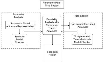
In this dissertation, we advocate the use of Parametric Timed Automata (PTA) to model real–time sys-tems. This approach allows us to represent a parametric real–time system retaining a large level of freedom on the specification of the activation and of the interaction patterns of the different tasks in the system. In this setting, the violation of temporal properties is encoded as a reachability problem of one or more undesired locations. For this problem, we develop an algorithmic solution, the Parametric Verification of Temporal Properties (PTVP) algorithm, that used a symbolic model checker to derive linear constraints for the task parameters that solve the reachability problem. The obtained linear con-straints are then used to construct the infeasible region of parameter space and subsequently provide us with the feasibility region of the system. This idea is implemented in a tool, Quinq, that is based on the NuSMV [22] model checker. The tool offers a variety of possible options for modelling the system, which we display in their application to a set of meaningful case studies.
1.3
Research Contribution
The contributions we made during our PhD research are the following:
1.4. STRUCTURE OF THE THESIS 3
• Setting up a methodology, based on PTVP algorithm, which enables an effective computation of a region of parameters that respect some required properties;
• Implementation of the complete method in the tool Quinq
• Application of the method and using the tool in several case problems : periodic task system [21], heterogeneous system [39], and in collaboration with Modular Performance Analysis Toolbox (MPA) [53].
The application of the methodology defined in this thesis to a set of case studies is a result of the collaboration with different authors. In particular, the application to heterogeneous and distributed real– time systems is a result of the collaboration with Hoa Le and Roberto Passerone. The connection between PTA and MPA is the result of the collaboration with Alena Simalatsar and Roberto Passerone, and MPA developers: Kai Lampka, Simon Perathoner, and Lothar Thiele.
1.4
Structure of the Thesis
This thesis is organised as follows:
Chapter 2 We introduce the basic definitions and terminology that we will use for real–time systems and for their design cycle. We then formalise the problem that we will target during the rest of the thesis. In the interest of clarity, we also introduce some application scenarios that will guide as through the course of the thesis as running examples. Finally, we spell out the most relevant research challenges addressed by the thesis.
Chapter 3 We offer an overview of the background knowledge that we used as the foundation of our work in this PhD dissertation.
Chapter 4 The parametric timed automata (PTA) model that will be the cornerstone of our thesis is introduced here. The analysis method that is used to check the parametric feasibility of a real–time system presented using PTA, our PTVP algorithm, is outlined in its main conceptual components.
Chapter 5 We analyse in detail the general architecture, and the different components required by the PTVP algorithm and by its implementation in the Quinq tool.
Chapter 6 We present two example applications of the tool: analysis of real–time periodic task sets with offsets and analysis of a distributed real–time system with flexible real–time constraints.
Chapter 7: the interaction of the tool with MPA is presented here as a paradigm of possible synergies with existing tools.
Chapter 8 Describes the related work on the verification of real–time systems with a particular focus on the tools and methodologies that carry out some form of parametric analysis.
Chapter 2
Real–time Design Challenges
2.1
Real–Time System
In a real–time system, the correctness of the results heavily relies on its timing performance. A failure in delivering the result within a specified temporal constraint (deadline) will make it useless in spite of its correctness. The ability for a system to meet its temporal deadlines largely depends on how shared resource are scheduled when more than one task compete for their access. For this reason, we will use the termschedulabilityto refer to the ability for the system to comply with its timing constraints for a given scheduling policy.
Real-time systems are pervasively present in our daily life. The range of their applications extends from the menial system to such critical systems as the anti-lock braking system (ABS) of the automobiles. Despite their pervasiveness, they often go unnoticed: as long as no violation of their required behaviour occurs, we will always have seamless systems in our hands.
The importance of correct real–time system
1. Safety Consideration
Examples of safety critical real–time systems are the control system of cars ( e.g., the fuel injection control, the ABS, the ESP) and of aircrafts, where a control system supervises the landing and take off process. For these systems, it is important that not even a single deadline is missed, as people safety depends on the correctness of the timing behaviour.
2. Manufacturing consideration
The embedded systems are usually mass-manufactured to reduce the production cost to the min-imum. A failure of a system that is only detected after the manufacture completes will cause a massive recall of the product, which determines potentially relevant economic losses. For this reason it has to be guaranteed that the system iscorrect by designbefore going into production. Current real–time system are increasingly variable in their behaviour and have to meet changing environmental constraints. Indeed, at run time, there can be many factors from the environment affecting the system. For this reason, some assumptions that have been made at design time might be violated during the system execution. In this case, the system is required to maintain its functional correctness and the timely delivery of the result. In other words, modern applications are required to berobustacross a wide range of operating conditions. In this context, a correct real–time system design flow is one that guarantees both the correctness and the robustness of its final outcome.
2.1. REAL–TIME SYSTEM 5
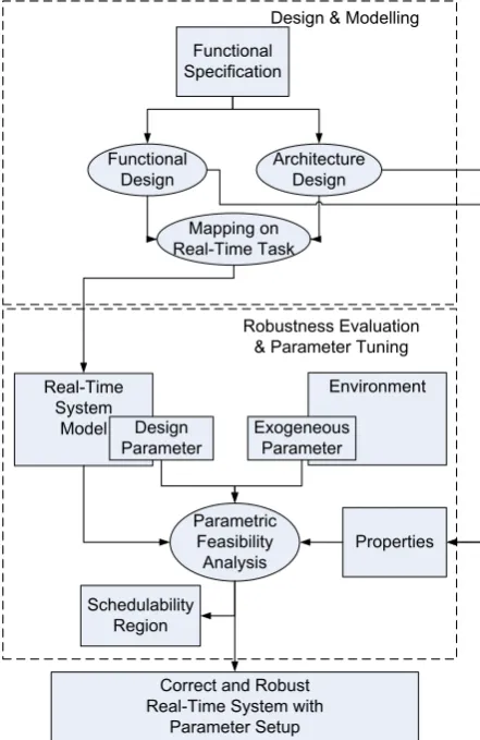
Figure 2.1: The design process of correct design
Designing Real-Time System
The methodology we envisage to achieve the goals discussed above is illustrated in Figure 2.1. The development process could be divided to the following two parts:
1. Designing and modelling
In designing real–time systems we start from the functional specification of what the system will do. This functional specification then will be implemented through functional designand archi-tectural design. Functional design specifies subfunctions which, in their interaction, will deliver the functionality. The architectural design specifies the hardware architecture and software infras-tructure that will be used for the real–time system. Based on the two designs, the subfunctions will be then mapped to real–time tasks making up the real–time system implementation. The mapped
real–time system modelhas to capture the following aspects:
2.1. REAL–TIME SYSTEM 6
(c) The scheduling algorithm : How we would schedule the execution of each subfunction when they compete for the same resource?
2. Robustness evaluation and parameter tuning
After constructing a model of the real–time tasks system, the next step is to asses its schedulability and robustness. In general, the designers need to do the following :
(a) Assign values for the quantities that fall within the designer control but that are not forced to take a pre-assigned value.
(b) Evaluate the system robustness with respect to the quantities that are not under control. Generally speaking, the model of the system comprises a set ofdesign parameters. These variables come from their activation pattern and timing properties of the tasks. For periodic tasks with offsets, design parameters the task periods, the deadline, the computation time and the offset time. Some of these parameters are under our control, some others are already fixed as they are dictated by the choices in the architecture design (e.g., the computation time). From the environment we will also have exogenous parameters, that is the external factors that will affect our system during the runtime. For example in a case where an aperiodic task is triggered by an event in the environment, the inter-arrival time between two adjacent events can be considered as an exogenous parameter.
Generally speaking, the correctness of a real–time system is evaluated on the ground of its ability to respect certainpropertiesthat derive from its functional and architectural design, first and foremost its schedulability. Therefore, designers are confronted with the problem of assigning the free parameters so that the desired properties are fulfilled and that the robustness of the system against possible variations of the uncontrollable parameters is maximised.
This leads us to the problem ofParametric Feasibility Analysis, which is the main objective of this work. In our view, the system is a multi–dimensional object, where each parameter is associated with a different dimension. In this context, performing Parametric Feasibility Analysis amounts to finding the region in in the multi dimensional space of the parameters such that every point in the region corresponds to an instantiation of the system that respects the required properties. We will refer to this region as thefeasibility region. This region will support the designer in tuning the parameter towards the desired level of robustness, leading him/her to the design ofa correct and robust real–time system.
What this thesis is about and what is not
To further clarify what we mean, it is useful to mention several possible queries a designers may raise in the design process. Among the several possible queries one might want to address in this first phase of the design are the following:
• Should single or multiple processors be used for the system?
• What priority should we assign to each tasks?
• Is it be possible to have the system distributed in several devices that then communicate?
2.1. REAL–TIME SYSTEM 7
This type of queries are important to map the functionalities correctly and as efficiently as possible according to the available hardware and software infrastructure. However, they are out of the scope of our thesis. Next, after the mapping of the system, we will need to assess the robustness of the system. We will encounter queries on robustness of the system, such as:
• How much could the computation of a task (or multiple tasks) can be stretched without affecting the system schedulability?
• With a distributed scheme is it possible to guarantee that the communication between the parts will respect certain timing latency criteria?
• Would it be possible for us to add one or several new tasks without affecting the system schedula-bility?
• How badly would such introduction of new tasks affect the robustness of the system?
• How could we tweak the offset to make the system schedulable?
Queries on robustness like these are the types of queries related to parametric analysis of the system. To answer queries such asCould we tweak into the offset to make the system schedulable?for example, we need to introduce the offset of the system tasks as parameters. That way in the parameter analysis of the offset we would be able to see which offset valuation would make the system schedulable. This is the kind of queries that we are interested in.
2.1.1 Terminologies and Definitions
In this section we introduce some basic terminologies and a set of definitions that we will use throughout our discussion.
Task model
A real-time systemsS is in our framework defined as a set of computing activities, henceforth referred to as tasks. Ataskorprocessis an entity of computation executed by an operating system. A real–time system consists of several tasks. For a generic task we will use the symbolτi, hence
S ={τ1, τ2, . . . , τn}.
Activation pattern
Each taskτiis characterised by anactivation pattern, a certain designed relative deadlineDi, and a worst
case execution timeCi. A taskτi generates a possibly infinite stream of jobsJi,1, Ji,2, . . .. Each job
Ji,1is characterised by [31]:
1. arrival timeai, j : the time when the job is activated or released so that it is ready for execution
2. start timesi, j: the time when the job is actually started being executed
3. finishing timefi, j : the time when the job finishes its execution
4. absolute deadlinedi, j = ai, j +Di : the limit time before which the job must have finished its
2.1. REAL–TIME SYSTEM 8
Figure 2.2: Figurative description of real-time job characteristic [31]
There’s also the notion of slack timeslacki=di−ai−Ci: the maximum time a task can be delayed
on its activation to complete within its deadline.
An activation pattern is a rule to generate the sequence of ai j. Possible examples of activation
patterns are:
Periodic the sequence is constructed as follows:
ai, j =φi ifj= 0 ai, j =ai, j−1+Ti ifj >0.
In this caseTiis saidperiodandφiis saidoffset. Sporadic the sequence is constructed as follows:
ai, j =φi ifj= 0 ai, j ≥ai, j−1+Ti ifj >0.
In this caseTiis saidminimum inter-arrivaltime andφiis saidoffset.
In this work we will more generally consider an activation pattern driven by atimed-automatathat we will specify in the next chapter. This is because in reality there are a lot more possibilities in activation patterns than the few just introduced. An example of a complex activation pattern task is given in fig-ure 2.3. We will enter into the details of the timed automata modelling later on. For the moment being, it suffices to say that this figure describes a task which is first activated after an offset timeO1 and then
after periodQ2. Afterwards, non-deterministically, it could either wait for an event or for timeQ1to be
activated, before waiting for the period ofQ2again.
From this simple example, we can easily see that periodic and sporadic patterns are special cases of timed automata driven activation.
Timing Properties
Real–time tasks can be further classified according to the criticality of their timing constraints. In partic-ular, we can introduce the following taxonomy of timing constraints:
1. Hard deadlines
An hard deadline requires that all for all the jobsJi, j activated by taskτi we havefi, j ≤di, j. A
2.1. REAL–TIME SYSTEM 9
Wait_for_ time_Q2
clock <= Q2
1 clock = O1 clock := 0 Wait_for_
offset clock <= O1
1 clock = Q1
clock := 0
2 clock = Q2
clock := 0 Wait_for_
time_Q1 clock <= Q1
3 clock := 0
Wait_for_ event
2 clock = Q2 clock := 0
Figure 2.3: The example of task with complex activation pattern
2. Soft deadlines
For a soft deadline, some failures can be tolerated up to certain extent. The completion after a deadline decreases the task performance, however it does not entail serious harm to the system. System such as in-flight entertainment system have this characteristic. The overall performance of the audio or video could get poorer on cases where some deadlines are missed, but this will not bring serious effects to the safety of the passengers. The respect of a soft deadline can be measured in probabilistic terms. This opens up the possibility of providing probabilistic real–time guarantees. We can require that the probability of respecting the deadline be grater than a specified value,P rob(fi, j ≤di, j)> µ, meaning that the percentage of possible deadline failures in the task
execution will be bounded byµ. This marks a big difference between a soft real–time task and a best effort task, for which no guarantee whatsoever is offered on the timing performance of the system [16].
3. Firm deadlines
As in the case of soft deadlines, some failures are tolerated for a firm deadline. However, the re-quired temporal guarantees are expressed in a deterministic fashion. Instead of using probability, the failure measurement can be expressed as the maximum number of deadlines that can be vio-lated consecutively until the system is deemed failed. For example, a system could tolerate up to two consecutive missing deadline events, retaining its functionality in spite of a decreased perfor-mance. However, if more than two consecutive deadlines are missed the system will no longer be functioning properly. We categorise this type of constraints as firm deadlines [43].
Interaction between tasks
2.1. REAL–TIME SYSTEM 10
Some systems require that a job of a task can be activated only after another job of another task terminates. This could happen because a task needs the output of another task as its input. This type of precedence relation is usually described through a directed acyclic graph (DAG).
2. Resource constraints
Some tasks require, for their execution, access to mutually exclusive shared resources. This type of access is usually supported by appropriate primitives of the Operating System such as mutex region, or semaphores. These shared resources could be a data structure, set of variables, memory area, or set of registers. The access to mutually exclusive resource requires ablockedstate for the tasks. The presence of a blocked state is important for the real–time performance of the system since it potentially introduces priority inversion [49]: a situation where a real–time task can be delayed for an arbitrarily long time by tasks having a smaller priority.
We define a real–time system as composed ofindependent tasksif all of its tasks have neither prece-dence constraints nor resource constraints. Most of the application that we will discuss in this thesis cover systems with independent tasks. However, our methodology allows for modelling certain types of precedence constraints between the tasks.
Schedulability of Real–Time System
Because tasks in a real–time systems are allowed to have overlapping execution requests that can exceed the number of available processing units, ascheduling policyis required. A scheduling policy is a set of rules whereby the operating system decides, for any point in time, which of the competing tasks should be granted the access to the processing unit. Ascheduling algorithmis the algorithmic translation of a scheduling policy. Ascheduleis an assignment of tasks to the processor such that each task is executed until completion.
As we are mostly focusing on the feasibility of hard real–time systems, the key property of interest is the following:
Definition 2.1. A taskτiis said to behard real–time schedulableif for all activation patterns of the tasks
in the system and for all the jobsJi, j, we havefi, j ≤di, j. The systemSis schedulable if all tasks are
hard real–time schedulable.
The problem in every real-time system is how to arrange all the real-time tasks involved in a schedule so that the system is schedulable. In the rest of the thesis we will use the termsschedulableandfeasible
interchangeably most of the times since schedulability will be the focal point of our interest. In some limited cases we will consider the combination of schedulability with other property of interests. In this case the term feasibility will take a broader meaning, but this will be clear in the context of the discussion. Further, unless specified otherwise, when we are discussing about schedulability, we refer to the schedulability in hard real–time sense.
In a real–time systems compounded of independent tasks, a taskτimight be not schedulable for the
following reasons:
1. the task execution requirements exceed the power of the CPU, e.g.,∃jsuch thatai,j +Ci≥di, j.
2.1. REAL–TIME SYSTEM 11
When tasks interact, a task’s schedulability could be affected by the blocking time on shared resources. In a firm real–time system, the schedulability property can be defined as follows :
Definition 2.2. A taskτiis said to befirm real–time schedulableif, for all activation patterns of the tasks
in the system, givennadjacent activationsJi, j we have at mostmtimes offi, j > di, j. The systemSis
schedulable if all tasks are firm real–time schedulable.
Scheduling algorithm
Central for the attainment of the schedulability properties is the selection of the most appropriate schedul-ing algorithm. Different families of schedulschedul-ing algorithms can be identified usschedul-ing the followschedul-ing classifi-cation [31]:
1. non preemptive: the scheduling algorithm is not allowed to interrupt the execution of a task: once it is assigned the CPU the task runs to the completion of the job;
2. preemptive : an executing task can be interrupted to yield the processor to another active task that, in that specific moment, has gained a higher priority;
3. static: all parameters (including the scheduling priority) are assigned to tasks before their activa-tion;
4. dynamic: the task parameters can be changed during its execution; therefore a task can have its priority raised or decreased in different moments;
5. offline: the schedule is decided before the task activation; 6. online: scheduling decisions are taken at at run-time
The policy to decide changes in the task scheduling priority is deeply influenced by the scheduling algorithm. For instance, if jobs have a long duration, the choice of a non-preemptive and on-line policy virtually nullifies the assignment of priorities. For online algorithms with static parameters the rate monotonic assignment (i.e.., priority growing with the activation rate) is known to be optimal if the tasks are activated periodically and if deadlines are equal to the period [42].
Task states
The presence of a scheduler requires to associate a task with a state. The possible states are the following: 1. active: a task that can potentially be executed
2. ready : a task waiting for the processor availability 3. running: a task in execution
The possible transitions between these different states are shown in Figure 2.4. First from being inactive a task will be activated when an appropriate event is triggered. After its activation, the task will be in
2.2. SCHEDULABILITY AREA PROBLEM FORMULATION 12
Figure 2.4: The different states of a task
2.2
Schedulability area problem formulation
We are now in condition to formally state the problem addressed in this thesis. First, we need to define design variables and parameters.
Design variables and parameters
As mentioned above, each task in an application can be associated with a set of parameters. Part of them are ground to a fixed value by prior design choice (e.g., the activation time of a control task could be imposed by considerations that have to do with control engineering). The typical real–time scheduling problem are formulated in the case of ground parameters. For instance, considering the case of periodic task sets the typically schedulability problem that can be formulated takes the following form:
Problem 1. Consider a task setS = {τ1, . . . , τn} scheduled with a given scheduling algorithm and periodic activation pattern. Assume all the tasks have agivenworst case execution timeCi. Decide whether or not all tasks are schedulable.
In this scenario, we consider a scheduling algorithm that allows preemption and allocates the CPU to the task using a fixed priority policy.
In the industrial practise, the designer could have a certain freedom of choice for some parameters. We will refer to these as “design parameters”. An example, could be the activation offset of the task, which can sometimes be tweaked to improve the system schedulability. In addition, other “exogenous parameters” have an inherent variability (e.g., due to an insufficient knowledge or to environmental conditions).
2.2. SCHEDULABILITY AREA PROBLEM FORMULATION 13
Figure 2.5: The example of the feasibility regionR
For instance we could have variable offsets for a periodic task execution. Generally speaking we asso-ciate to each taskτi a vectorρi of design parameters (e.g., for a periodic task with offset this vector is
given by:ρi= [φi, Ci]).
If the role of parameters is considered a problem like Problem 1 takes a different and more general form.
2.2.1 General Problem Formalization
First of all, it is possible to define the feasibility region as follows:
Definition 2.3. Consider a task setS ={τ1, τ2, . . . , τn}, scheduled by a given scheduling algorithm.
Let each taskτi be associated to a vector of design parameters ρi taking values in the setΓi and let ρ = [ρ1, ρ2, . . . , ρn]be a vector aggregating the parameters of all the different tasks. The feasibility
regionR ⊆ Γ1 ×Γ2 ×. . .Γn is defined as: ρ ∈ R if and only if the system is schedulable with the
choice of parametersρfor the different tasks.
The definition above leads us to the following formalisation.
Problem 2. Consider a task setS = {τ1, . . . , τn} scheduled with a given scheduling algorithm and with activation pattern of eachτi specified. Letρbe the vector of design parameters defined in the set
Γ = Γ1×. . .×Γn. Find the feasibility regionR.
The definition and the problem formulation above are easily generalised to systems using multiple types of resources (processors, communication links) and to the verification of more general temporal properties than the simple task schedulability.
Example 2.1. Consider the example of a task set S = {τ1, τ2} where τ1, τ2 are two periodic tasks
withT1 = 4andT2 = 8. Their deadlines are equal with their periods and their offsets are zero, i.e.,
D1 =T1= 4,D2 =T2= 8,φ1=φ2 = 0, and the design parameters areρ1 = [C1],ρ2= [C2]. In this
case the choice of parametersρ = [ρ1, ρ2]is described in the equation C41 + C82 ≤1[31]. Therefore
2.3. EXAMPLE SCENARIOS 14
2.3
Example Scenarios
To illustrate the potential applications of the methodology in a design flow for embedded systems, we propose a couple of simple possible real world design scenarios. Later on in the thesis, some of this scenarios will be reprised and used as a running examples for our discussion. In this context, we simply use them to outline the possible design issues that our methodology allows us to address and the type of results that can be obtained.
Scenario 1
Given of a real-time system with a set of periodic tasks and offset to each tasks arrival rate such as a control system in nuclear power plant. The timing deadlines are hard deadlines as this is a critical system. The tasks are scheduled using a pre-emptive scheduler with static pre-assigned priorities. The designer is required to maximise the system robustness, allowing the system to survive in case of unforeseen environmental disturbance that could affect its computation time.
We use a periodic task systemS1 = {τ1, τ2}. Periods are fixed and chosen equal to the relative
deadline:T1=D1 = 20andT2 =D2 = 30.
Use case 1:Consider a design scenario in which the computation times are not known with a sufficient precision and the system is very close to the border of the schedulability region found with traditional real-time scheduling theory (i.e., assuming null offset). The design problem is how to choose a pos-itive offsetO2 so as to maximize the schedulability region (and hence the robustness of the system).
Thereby, we aim to compute the schedulability region with respect to the following set of free parame-ters:{C1, C2, O2}fixingO1 = 0.
The application of the methodologies shown below in the thesis allows us to construct the region illustrated in Figure 2.6. We can see three different sections obtained by cutting the three-dimensional region with the planes O2 = 0, O2 = 5, and O2 = 8. In accordance with the notion of critical
instant from the classical real–time scheduling theory,O2= 0corresponds to the smallest schedulability
region. The choiceO2 = 8is the one that ensures the maximum robustness for the choice ofC1, while
O2corresponds to the greatest schedulability region.
Use case 2: Assume that the worst computation time of the tasks are fixed,C1 = 11andC2 = 12.
This task system is not schedulable with zero offsets as it is possible to see with a standard response time analysis as can be seen in the upper illustration in Figure 2.7 Therefore, we would like to identify the possible values for the offsetsO1andO2that make the system schedulable.
The region resulting from the application of our methodology is shown in Figure 2.8. Using the information from the figure we can then simply pick the values forO1, O2andO3inside the feasibility
region to makeS2 schedulable. We can choose O1 = 5and O2 = 1for example. And the system
will now be schedulable, in spite of a system utility close to 95% and to a non–harmonic choice of the periods.
Scenario 2
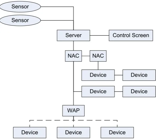
This example is inspired by the Heterogeneous Communication System (HCS) of a civil aircraft [27]. The problem is to stream the audio package and synchronize them. The architecture of the system is shown in Figure 2.9.
2.3. EXAMPLE SCENARIOS 15
1 3 5 7 9 11 13 15 17 19 21 23 25 27 29
1 3 5 7 9 11 13 15 17 19 21 Region with O2= 8
Region with O2= 5
Region with O2= 0
Or O2= 10
Figure 2.6: Feasibility regions of Scenario 1, Use case 1,in the domain ofC1andC2for different values
ofO2
1
2
3
4
5
6
7
8
9
10
0
Task 1
Task 2
Task 3
Task 1
Task 2
1
5
10
15
20
25
30
Task 1
Task 2
1
5
10
15
20
25
30
Figure 2.7: In the upper figure the system will fail usingO1 =O2 = 0, while in lower figure the system
2.3. EXAMPLE SCENARIOS 16
1 3 5 7 9 11 13 15 17
1 3 5 7 9 11 13 15 17
19
Figure 2.8: Regions of feasibility in the domain of O1 and O2 for Scenario 1, Use case 2.
devices implement also the Precision Time Protocol (PTP) [47] to synchronize their clocks.
The communication between the server and device is asynchronous. The server sends an audio packet everyaudP eriodms; audio packets are characterized by two parameters: a sequence numberi
and a timestamptidenoting the time the packet has to be played at the device. Due to varying network conditions, packets arrive at the device (except if they are lost) with a minimal latency Lmin and a maximal latencyLmax. The NACs simply forward the incoming packets to the devices. Packets passing through the NACs experience delay of Lnacduring which they are preprocessed by the NACs. The device processing time for each audio packet isτ, after which the device is ready to receive the next audio packet. The PTP protocol runs on the server, the devices and NACs, and is used to synchronize the respective clocks. The audio packets have firm deadline requirements. A packet may miss its deadline as long as the previous packet has not already missed the deadline.
Various timing delays are to be guaranteed, for example, in a scenario where two devices are con-nected to the server, it should be guaranteed that both devices are synchronized within an error of0.1ms (synchronization precision).
In this system the parameters that we can play with for example are the buffers used, the latency
LminandLmaxin the medium and alsoLnacin NAC, the computation time of each processes, and the clock driftcwhich is the offset time of the local clock compared to the server clock. The properties that we can check are for example:
• Whether or not buffer overrun could happen.
• That the firm deadlines of the audio packets are not missed
2.3. EXAMPLE SCENARIOS 17
Figure 2.9: Heterogeneous Communication System (HCS)
• Can we tweak the computation time of task to enable maximum robustness of system schedulabil-ity?
The objective of this work is to answer the last query for example by something like is shown in Figure 2.10, where we can see the possible values for the computation time that will ensure the schedu-lability on different values of clock drift∆.
Scenario 3
Consider a real–time system with CPUs whose speed changes with the size of the backlog buffer. The scheduler of the example load-dependent frequency adaptation scheduler is adapted from [35]. The scheduler can change its processing speed when the number of tasks in the buffer has exceeded certain threshold. The tasks are activated periodically with jitter. However, unlike in the previous scenarios, the task activation and the result in this case is represented through timed automata that producesstream.
A stream is characterized by a pair of so called arrival curves [52]. These arrival curves bound the number of activation events for any interval∆ ∈ [0,∞). Thus arrival curve is characterized by the maximum number of tasks in burst and the widths∆of the stairs. We need to capture the system behaviour given the input and output of the system in terms of the arrival curve.
The parameters that we could play with in this kind of systems are the maximum number of tasks in burst on the input and or the output of the system, the widths of input/output curve stairs, maximum latency that can be tolerated for each task activated, and its maximum buffer size.
2.4. CHALLENGES 18
0 2 4 6 8 10
0 2 4 6 8 10
C2
C1 ∆=0
∆=3
∆=5
∆=7
Figure 2.10: Audio feasibility and error regions for∆ = 0,3,5,7.
2.4
Challenges
Concluding from the illustrations in the scenarios presented previously, here are the challenges that we need to handle in designing real–time sytem.
1. Providing model that could represent general activation pattern of tasks and scheduling require-ments and policies.
2. Performing the schedulability analysis for all possible design parameters
Our main challenge is to have a tool that is able to answer both challenges we presented above. In our research we need to handle these outstanding issue on the model and the method that we will use to analyse the feasibility of a system:
• Model
The model that we use need to fulfil the following criteria: 1. Expression power
The model should have strong expressive power to be able represent general real time system. 2. Usability
The model should be easy enough to use by designers that have no in-depth knowledge of formal methods.
3. Tractability
The model should be tractable as in having other use other than just plain for modelling. For example it could also be used as problem presentation.
• Verification Method
2.4. CHALLENGES 19
1 2 3 4 5 6 7 8 9 10
1 2 3 4 5 6 7 8 9 10 DeltaOne
Unschedulable region
BMAXOne
Chapter 3
Background Knowledge
3.1
Satisfiability Modulo Theory
3.1.1 Logic Terms
First, we enumerate several definitions that we will use in discussing the topic of Satisfiability Modulo Theories (SMT) and logic in general.
Propositional Logic
We start from the most basic building block of logic formulas: propositional variable. Apropositional variableis a variable with value of eitherTrueorFalse. Apropositional formulaϕis built from propo-sitional variables. It can consist of one propopropo-sitional variablep, or a negation¬ϕ0, conjunctionϕ0∧ϕ1,
disjunctionϕ0 ∨ϕ1, implicationϕ0 → ϕ1 or bi-implicationϕ0 ↔ ϕ1 of other propositional formula
ϕ0 andϕ1. A literal is a propositional variable por its negation. Literals are connected by disjunction
to form a clause. We say that a formula is in conjunctive normal form (CNF) if it consists of clauses connected by conjunctionC1∧. . .∧Cn. Any formula can be made into a CNF formula.
Atruth assignmentM for a formulaϕassigns all the propositional variables inϕto eitherTrueor
False. A truth assignmentM satisfiesϕ, with the notationM ϕ, if the assignments of values inM
makesϕTrue. A formulaϕis satisfiable if there is anM that could satisfy it,M ϕ.
EXAMPLEGiven a formulaϕ= (p∧ ¬q)∨r, the truth assignment
M ={p7→T rue, q 7→F alse, r7→F alse}satisfiesϕ.
Satisfiability Problem
Given a propositional formula, the satisfiability problem amounts to deciding if there is a modelM that satisfies it. We call this specific problem aspropositional satisfiability SAT problemor shortly asSAT problem. The solution of a SAT problem is NP-complete.
First-Order Logic
First-order logic extends the propositional logic with functions, predicates and quantification. The basic entities in first-order logic are terms. Atermtcan be a constantc, a variablexover a certain domain, or a function whose arguments are terms. The notation for an n-ary functionf isf(t1, . . . , tn). Predicates
3.1. SATISFIABILITY MODULO THEORY 21
can be seen as functions that return eitherTrueorFalse. A predicate describes the relation between its arguments. For exampleP(x, y)could meanxsmaller thanyandQ(y)could meanyis a female.
Aformulais a predicatep(t1, . . . , tn)or negation ¬ϕ0, conjunctionϕ0∧ϕ1, disjunctionϕ0∨ϕ1,
implicationϕ0 ⇒ ϕ1, bi-implicationϕ0 ⇔ ϕ1, and quantification∀xϕ0 or∃xϕ0 of other formulaϕ0
andϕ1. AΣ-formulaϕis a formula with all the symbols defined in the domainΣ. Afree variablexinϕ
is a variable that is not bounded by any quantifier∀or∃. Asentenceis a formula without free variables. AmodelM is a set of interpretation of all the variables, functions, and predicate symbol that makes the formulaϕTrue. A formula is satisfiable is there is a modelM that could satisfy it,M ϕ.
Theory
AΣ-theoryis a set of sentences overΣ. The satisfiability of a theoryTisdecidableif there is a procedure that determines the satisfiability of any quantifier-free formula in it. Linear Arithmetic theory for example is the theory with functions+and−applied to either numerical constants or variables, and multiplication between a constant and a variable. The predicates of this theory are=, <,≤. Given a linear arithmetic formula, its satisfiability can be decided by using dual simplex algorithm for formula with = and ≤
predicate and by using the algorithm extension for formula with strict inequality< predicate. Since there exists this algorithm to determine the satisfiability of formula in Linear Arithmetic theory, this theory is decidable.
Example 3.1. We provide an example formula of first-order logic over linear arithmetic. The formula ϕ = (x+ 2∗y ≤0)∧(x <0∨(2∗x+ 4∗y+ 2<0))is made of Boolean combinations of linear arithmetic constraints. The modelM ={x=−1.0, y= 0.5}satisfiesϕ. Thus, formulaϕis satisfiable.
3.1.2 Satisfiability Modulo Theory
Many of the industrial problems require the expressive power of first order logic. Aside from simple declarative propositions, predicates and quantification are usually needed. And, instead of having all boolean variables an industrially relevant problem could have a mix some real and or integer variables and some arithmetic operations. For instance, in our problem specification in modelling real– time system, we need to include the notion of continuous time in the environment as the rationals factor in the formula.
Linear programming algorithms can check the satisfiability of conjunctions of linear arithmetic in-equalities, but they can not be applied directly to Boolean combinations. For this kind of problems we define the notion of Satisfiability Modulo Theory (SMT). A formulaϕissatisfiable modulo TifT∪ϕis satisfiable. Referring to the problem in Example 3.1 the formula is satisfiable modulo linear arithmetic theory if the formula made of the union of solving the arithmetical constraints in the theory of linear arithmetic and the boolean parts ofϕis satisfiable.
Generally, SMT is a decision problem involving various theories which are expressed as simple first-order logic. SMT solvers work by combining special purpose algorithms for each domain. Example of these theories are, e.g., the theory of difference logicDL, the theoryEU Fof equality and uninterpreted functions, and the quantifier-free fragment of Linear Arithmetic over the rationalsLA(Q)and over the integersLA(Z)[15]. This enables a richer representation than simple boolean SAT formulas.
3.1. SATISFIABILITY MODULO THEORY 22
Figure 3.1: A simple description on SMT solving schema
a SAT solver to solve the Boolean parts of the formula, and of Theory solver(s) to solve the other logic problems involved. The interaction between the two class of solvers is illustrated in Figure 3.1.1.
An SMT-solver first will extract the Boolean skeleton on the input formula. This is obtained by replacing the theory constraints in the formula with auxiliary Boolean variables. Given the Boolean skeleton formula ofϕ, SAT solver performssystematic searchin a tree of which each vertex represents a propositional variables and the outgoing edges representTrue andFalse. This systematic search is performed to find a truth assignmentM that will satisfy the Boolean skeleton ofϕ. Most search based SAT solvers are currently using DPLL approach. While the SAT-solver tries to construct a satisfying assignment for the Boolean skeleton of the SMT formula iteratively, the theory solver then verifies the conjunction of the constraints which have to hold according to the so far constructed assignment.
Example 3.2. We refer to the example problem given in example 3.1. If we replace each of the arith-metical constraints inϕ= (x+ 2∗y≤0)∧(x <0∨(2∗x+ 4∗y+ 2<0))by a Boolean variable we will obtain the formulaA∧(B∨C) as the Boolean skeleton ofϕ. First the SAT Solver will try to assignA 7→ T rue. This will send the constraintx + 2∗y ≤ 0 to the theory solver. Theory solver will check its consistency to theTrueassignment and will report that it is satisfiable. SAT solver then continues to assignA 7→ T rue, B 7→ T rue, C 7→ T rue. The rest of the formulaϕis now sent to the theory solver. The theory solver will report unsatisfiability and give back the constraint A,x+ 2∗y≤0, and C,2∗x+ 4∗y+ 2 <0, as reasons. The SAT solver uses this information to undo a part of the current assignment (backtrack), learn that it should not assign both A and C to True, and continue the search.
3.1.3 Bounded Model Checking
The approach we used in this work to carry out the verification process of SMT is symbolic and is based on bounded model checking (BMC) method [9]. The verification of the timed system is done by considering a finite and increasing time bound. In each iteration, the verification problem is transformed into the satisfiability problem of a set of formulas defined over boolean variables and real variables. We will provide an example of how a timed automata is unrolled step by step for BMC on the timed automata section example 3.4.
1
3.1. SATISFIABILITY MODULO THEORY 23
The result of the BMC is a satisfiability response or a counterexample. Namely, for a finite transition systemM the property of interest is the satisfiability of a Linear Time Logic (LTL) formula ϕ. For a given number of stepsk, the model checker searches for counterexamples of lengthkas the bound, and decide thatMsatisfiesϕiff there is no counterexample exists in the path of lengthkor less than k.
The most important problem of BMC is to identify a number of stepsCT such that if no counterex-amples are found within the boundCT thenM|=ϕ(the formula is satisfied). Such problem is defined as the Completeness Threshold (CT)problem. In [24] a computation method to find an upper bound ofCT is described for the reachability problem on finite systems. The bound is sufficiently computed by finding the initialized diameterdI(M), which is the longest shortest path from an initial state to any reachable state ofM. Using B¨uchi Automata with Vardi-Wolper LTL model checking framework it is found that such value ofCT is computable with a formula of sizeO(klogk). An important open issue is to verify whether a similar notion on the computability ofCT can also be applied to timed automata.
A problem with the theoretical bound just mentioned is that it tends to be un-necessarily large. In practical cases, the maximum length of a possible counter-example for the property of interest can be much shorter. Very useful in this respect is to complement BMC methods with inductive reasoning. Inductive reasoning is a reasoning method which work on verifying that the initial state satisfies property
ϕ, and from all the steps from 0 to kthat verifies the property, we can only go to stepk+ 1 that also verifies the property. Optimizing BMC with inductive reasoning we could verify if no counter example is found at stepkthen we will not found it onk+ 1step, thus providing termination result to the BMC search.
3.1.4 Tools
One of the tool developed to decide the satisfiability of theories problem belonging to the category of SMT is MathSAT [13]. MathSAT solves this problem based on Davis-Putnam-Logemann-Loveland algorithm (DPLL), which decides the satisfiability of propositional logic formulae in conjunctive normal form(CNF) by using backtracking decision procedure, and it is able to solve SMT problem for various theories. One of them, which is important for our purposes, is Linear Arithmetic over the Reals (LA (R)). The ability to solve problems based on this LA (R) theory encouraged the use of MathSAT in this work.
This MathSAT is a foundational tool for NuSMV3, the latest version of NuSMV [22], a verification tool that combines the strengths of Binary Decision Diagrams (BDDs) of NuSMV and SMT solvers of MathSAT. NuSMV itself is a reimplementation and extension of SMV symbolic model checker, the first model checking tool based on Binary Decision Diagrams (BDDs). BDD is a data structure that is used to represent a Boolean function. Abstractly, BDDs are as a compressed representation of sets of boolean functions. However, unlike other compressed representations, operations are performed directly on this compressed representation, thus minimizing the complexity.
The extension of NuSMV to NuSMV3 entailed the definition of a language involving new types involving both Integer and Reals and hybrid automata. The full integration with MathSAT SMT solver has also enabled the construction of other model checking algorithms which were not in the initial dis-tribution of NuSMV. Most notably the model checking that we will use are Bounded Model Checking via SMT and Interpolation based invariant checking for induction. An extended set of features such as requirements analysis, dependability assesment, and safety analysis are also provided in this extension.
3.2. TIMED AUTOMATA 24
Wait_for_ period
x <= T1
y <= Timeout Release1 x = T1 x := 0
Release1
x = O1 x := 0
Wait_for_ offset x <= O1
Error Abort
y > Timeout
Reset y := 0 x := 0
Figure 3.2:T A1, an example of a task activation automata to be encoded in NuSMV.
analysis of timed automata.
3.2
Timed Automata
The notion of timed automata was first proposed by Alur et al. [1] to enable an explicit modelling of time, and it was later recognized as an effective formal notation to model the behaviour of real-time systems. A timed automata is a directed graph, in which nodes are called the locations and the arcs are called the transitions. Time modelling is achieved by the use of clock variables. The constraints on the values of the clock determine the temporal evolution on the timed automata.
3.2.1 Timed Automata Formal Notation
A timed automatonA [1] is defined as a tuple ofhL, L0,Σ, X, I, Eiand its components are defined as
follow:
• Ldefines the finite set of locations in the timed automata.
• L0⊆Ldefines the set of initial locations
• Σdefines a finite set of labels of events affecting the evolution of the timed automata.
• Xdefines a finite set of clocks
• I, describes the invariant of a location. It defines a mapping between each locations ∈ L with some clock constraint in the set of clock constraintsΦ(X)
• E ⊆L×Σ×2X×Φ(X)×Ldefines the set of switches. A switch with the formal representation
3.2. TIMED AUTOMATA 25
Example 3.3. We present in Figure 3.2 an example of timed automataT A1. The components ofT A1
are:
1. Li:L={W ait f or of f set, W ait f or period, Error}.
2. L0:L0 =W ait f or of f set.
3. Σ: The labels areΣ ={Release1, Reset, Abort}.
4. X: The clocks in this example areX ={x, y}.
5. I : We have the invariant for locationsW ait f or of f setandW ait f or period. We write them asI ={state=W ait f or of f set→(x≤O1)} ∧
{state=W ait f or period→(x≤T1∧y <=T imeout)}.
6. E: There are 4 transitions in our example, as we need to name each transition, we will name them with the following format
<origin_state>_<destination_state>_<transition_number>}
The set of transitions that we have is
E={wait f or of f set wait f or period 1,
wait f or period wait f or period 2, wait f or period wait f or of f set 3, wait f or period error 4, .
A system made of a set of automaton is defined as a product construction of the involved automata. Given two timed automataA1 = hL1, L10,Σ1, X1, I1, E1i andA2 = hL2, L20,Σ2, X2, I2, E2i.
As-suming clock setsX1 and X2 are disjoint, a product A of A1 and A2 is the timed automaton A =
hL1ף2, L10×L20,Σ1∪Σ2, X1∪X2, I, EiwithI(s1, s2) =I(s1)∧I(s2). The switches are :
1. h(s1, s2), a, ϕ1∧ϕ2, λ1∪λ2,(s10, s20)i, fora∈Σ1∩Σ2and for everyhs1, a, ϕ1, λ1, s10iinE1
andhs2, a, ϕ2, λ2, s20iinE2.
2. h(s1, t), a, ϕ1, λ1,(s10, t)i, fora ∈ Σ1\Σ2 and for everyhs1, a, ϕ1, λ1, s10i inE1 and everytin
L2
3. h(t, s2), a, ϕ2, λ2,(t, s20)i, fora ∈ Σ2\Σ1 and for everyhs2, a, ϕ2, λ2, s20i inE2 and everytin
L1
Thus, a transition of A is obtained by coupling the transitions of the individual automata labelled with consistent event sets. A special type of transition that preserves clocks and locations is defined asstutter transition. An automata takes the stutter transition when a transition takes place in another automata that is not synchronized with any of its label.
A run of timed automata consists of states and transitions between them. A state is(s, ν), withs∈L
andνassignment to the clocks such thatν |=I(l). A state is an initial iffs∈L0 andν(x) = 0for all
clockx∈X.
3.2. TIMED AUTOMATA 26
Wait_for_ period
x <= T1 y <= Timeout Release1 x = T1 x := 0
Release1
x = O1 x := 0
Wait_for_ offset
x <= O1
Error Abort
y > Timeout
Reset y := 0 x := 0
Wait_for_ reset x1<= Treshold Release1
x1:= 0
Idle
Reset x1<= Treshold
Release1
Figure 3.3: A timed automata to be encoded in composition withT A1
1. Discrete transitions
It is a transition that happens when in the state(s, ν)a switchhs, a, ϕ, λ, s0isuch thatν |= ϕis taken. We write this(s, ν)−→a (s0, ν[λ:= 0]). Stutter transition is also categorized in this class. 2. Continuous transitions
Defined asδ-transitions, they represent the time elapse in the timed automata system. For a state
(s, ν) experiencing time elapseδt ≥ 0, we write(s, ν) δt
−→ (s0, ν +δt)if for all 0 ≤ δt0 ≤ δt, ν+δt0 |=I(s). The time elapse transitions are synchronized on all timed automata in a system.
A run of length k is a sequence of states (l0, ν0),(l1, ν1), . . . ,(lk, νk) iff the first state is initial, and fori = 0, . . . , k −1 it holds that (li, νi) −→σ (li+1, νi+1) for some switch σ, or li = li+1 and
(li, νi)−δ→t (li+1, νi+1).
Example 3.4. To describe the composition of automata and the run of automata, we present the second exampleT A2 in Figure 3.3 which will be synchronized with T A1, our previous example in figure 3.2.
This timed automataT A2 synchronizes with T A1 on the event of Release1. After the first event of
Release1, within timeT hreshold,T A2could non-deterministically fire theResetevent.
Using the following assignment{T1 = 4, O1 = 2, T imeout= 9, T hreshold= 5}, then one of the
possible run for the automataT Awhich is the product of timed automatonT A1in Figure 3.2 and timed
automatonT A2in Figure 3.3 is:
((WFO,Idle),{x= 0, y= 0, x1 = 0})
δ2
−→ ((WFO,Idle),{x= 2, y= 2, x1 = 2})
Release1
−−−−−→
((WFP,WFR),{x= 0, y = 2, x1= 0})
δ4
−→ ((WFP,WFR),{x= 4, y= 6, x1 = 4})
Release1
−−−−−→
((WFP,WFR),{x= 0, y = 6, x1= 4})
with WFO =W ait F or Of f setstate and WFP =W ait F or P eriodinT A1while WFR =
W ait F or Resetin T A2. The run above depicts how it starts in the initial location (WFO,IDLE)
which is made of the initial location ofT A1 andT A2. All the clocks,{x, y, x1}, which are the union of
clocks fromT A1 andT A2, have zero values in this initial state. The first transition is aδ-transition of 2
3.2. TIMED AUTOMATA 27
wait f or of f set wait f or period1inT A1andidle wait f or reset 1inT A2is enabled and taken.
This discrete transitions changes the location of the automata to(WFP,WFR)and reset the clocksxin T A1andx1inT A2while the clockyinT A1retains its value. Next, we have anotherδ-transition with 4
time units that increment all the clocks value. And now as the guard of transition with labelRelease1that
is composed ofwait f or period wait f or period 1forT A1 and stutter transition inT A2is enabled.
Taking this transition moves us to the next state where we stay in the same location(WFP,WFR)but the clockxofT A1has been reset while clockyandx1retain their values.
3.2.2 Timed Automata Verification in NuSMV
A first possibility for verifying timed systems is the application of such model checkers as UPPAAL2. This approach is taken in the TIMES tool [28, 29, 45], which is a derivation of UPPAAL specifically targeted to the verification of real-time scheduling properties. The approach can be classified as an explicit s
![Figure 2.2: Figurative description of real-time job characteristic [31]](https://thumb-us.123doks.com/thumbv2/123dok_us/639194.2063964/19.595.227.408.104.186/figure-figurative-description-real-time-job-characteristic.webp)