Modeling and Analysis of a
R
eal-time
S
ystem
Us
ing the
N
etworks of
E
xtended Petri
Mohammed Blej *,** * Laboratoire MATSI, UFR ANITS
** Faculté des sciences, Université Mohammed Ier, Oujda, Maroc Email: [email protected]
Mostafa Azizi *, ***
*** Ecole Supérieure de Technologie, Université Mohammed Ier, Oujda, Maroc Email: [email protected]
Abstract—In this paper, we propose to study and analyze the tasks of a robot and the interaction with its environment, by using the power of Petri nets modelling, especially the timed nets. Our system consists of a robot, a programmable automaton and a computer. We consider the execution of the tasks taking into account the temporal constraints. So, we use the temporal Petri nets to model the whole system and also for its verification. We describe the obtained Petri net and the constraints textually or graphically in the environment TINA, an open source tool dedicated for timed Petri nets. We note that the Petri nets have good qualities of abstraction from the modelling point of view compared to the finite state machines which suffer from the states explosion problem, related to the accessibility graph. Moreover, the consideration of the temporal constraints adds an important complexity to the problem; the system which was carried out successfully in the case "without temporal constraints", can get in a dead lock state in the case "with temporal constraints" if these constraints are not satisfied.
Index Terms—Time Petri nets, Tool TINA, Real time system, Task managing, Time constraints
I. INTRODUCTION
The tasks performed by a robot become increasingly varied and complex. Modeling a simple task and analysis of its evolution could lead to great satisfaction, but when combined with other tasks to form the complete system, the problem becomes quite rigorous, especially with the consideration of time constraints related to the functioning of the system.
Most work on the design tasks of one of several robots, using discrete event systems based on finite state machine [12, 18, 11, 9, and 2]. This technique is often confronted with the problem of so-called combinatorial explosion; through Petri net and its extensions to express specific time, we may conduct an analysis of a real-time system [13]. The Petri net owns a very important property of abstraction that can limit the problem of explosion. Our interest is then focused on the exploitation of the
expressive power of extended Petri net [13, 16] to test and verify the correct functioning of a real-time system. Such an analysis can be made a priori and a posteriori, depending on the system if it is already developed or being specified.
The rest of this article is organized as follows: The second section presents our approach of system analysis based on timed Petri nets using the services of the tool TINA. Before concluding, we discus in the third section the obtained analysis results.
II. APPROACH SYSTEM ANALYSIS
II.1. Petri Net
Among the existing models of discrete event systems, Petri net are widely used to model dynamic systems, especially automated manufacturing systems [20]. Their properties make them good candidates for performance evaluation, both qualitative and quantitative. For a formal definition of Petri Net (PN), the reader can relate to [6], [8]. A Petri Net is a bipartite graph consists of a set of places, transitions and directed arcs that connect the places to transitions and the transitions to places. It is represented by a quadruple <P, T, Pre, Post> where:
-P is the set of places, and T is the set of transitions. -Pre: P x T→Ν is the application corresponding to arcs that connect places to transitions. - Post: P x T→ Ν is the application corresponding to arcs that connect transitions to places.
A marked Petri net is a couple (R, M), where R is a Petri net and M is its marking that combines a number of tokens to each place of P.
II.2.Time Petri Net
These are nets where each transition has two dates min and max. Thus, if a transition T is sensitive for the last time at the date θ, then T can be fired before the date θ + min and must be no later than the date θ + max, unless the firing of another transition has desensitized T before it is fired [4]. We use in this case TINA [22] as an analytical tool. TINA (Time Petri Net Analyser) is a software environment for editing and analyzing PN and TPN [5]. There are two major extensions of Petri net that take into account the time aspect when modeling a real-time system: real-timed Petri nets [21] and Time Petri Net [19]. For the first extension, the timings are associated is the transitions (the net is said T-timed) or to the places (the net is said P-timed). The timing represents for a transition the minimum duration of its firing and for a place the minimum stay of a token within this place. The T-timed Petri are equivalent to timed ones, i.e. a P-timed Petri net can always be converted to a T-P-timed Petri net and vice versa. These are a subclass of Time Petri Net [7]. For the second extension, time intervals are assigned to transitions (T-timed net) or to places (P-time net). It has been shown in [17] that T-time Petri Net and P-time Petri are incomparable (not equivalent). These two models are a subclass of "Time Stream Petri Nets' [10] which were introduced to model multimedia applications.
A Time Petri Net is a 6-uplet <P, T, Pre, Post, m0, Is> where <P, T, Pre, Post, m0> is an ordinary Petri net and Is: T → I+ is a function that associates a time interval Is (t) to each transition of the net.↓Is(t) and ↑Is(t) are called static shooting dates of the transition t respectively as soon as possible (lower limit) and no later than (upper limit) [4]. A state of a TPN is a couple e = (M, I) where M is a marking and I: T → I+ a function that combines a time interval for each transition alerted by M.
II.3. Presentation of our system
Our studied system is composed of a computer (software) for supervision, a robot, and a programmable automaton for interfacing between the system and the robot (see Figure 1).
The used software determines the next N tasks for the robot (N fixed) and sends them to it through the automaton, with respect to the execution rate of the robot. If this later can not perform a submitted action, then the computer will be informed via the automaton. When the robot finishes properly performing an action, the automaton delivers to it the following actions.
The automaton reminds the computer, after submitting the last action to the robot, to supply the next jobs. We assume that the system is idle at the initial state, and then it starts. To stop it, the software sends a control message in stead of expected actions. Once the automaton received the message, it leads the robot to rest as soon as its current actions have been executed.
Figure1. Robot System
II.4. Modeling our system using Petri nets
We used for modeling of our system the method of scheduling a Petri net, presented in [14, 15]. As the system is composed of three entities, namely the robot, the automaton and the computer; each entity is modeled separately and then combined with others to rebuild the entire system. The robot faces three situations:
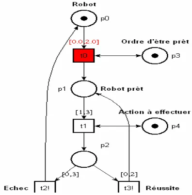
(1) "the robot is waiting for action" (2) "the robot is ready to perform an action" and (3) "the robot is in the process of performing an action "(see Figure 2). Each situation is represented by one place. Initially, the place P0 which represents the robot, contains a token otherwise the robot is defective and the system gets in a blocking state. The robot switches from one situation to another during its evolution in response to the messages received from the automaton, which is represented by the place p3. The robot communicates with automaton to receive the action to run, via the place p4. Transitions T2! and T4! indicate respectively the failure and the success of the robot operation. The robot may fail to do its tasks due to internal or external reasons, such as an obstacle; this is traduced by getting into specific places or by non respect of timed constraints.
On the other hand, the automaton switches between two situations: "waiting" and "active". The software is modelled by a Petri net of three places: the first one expresses that the computer is waiting; the second determines the actions to be performed and the third shows the process is running. We obtain the whole model of the system by the composition of the three Petri nets (see Figure 3).
We used TINA for performing a simulation of this system. TINA is an open source tool dedicated to the Petri nets, developed in Java, it can describe a problem in a Petri net, to carry out simulations, to calculate marking graphs and to test the presence of execution blockages.
Figure2. Petri net of the robot
III. DISCUSSION OF RESULTS
III.1. Methodology analysis
Our methodology for analysis of such a system follows the coming steps:
(i) Description of the three separate components of the system: we represent each component by a Petri net which describes its functioning (see Figure 2)
(ii) Unit testing: we conduct unit tests of the three Petri nets obtained from the stage (i). By performing these tests, we are looking to check whether each Petri net is working in accordance with the functional specification of this part of the system. Other properties of the Petri net are also generated, we cite as examples the properties of boundness and safety.
(iii) Composition of the three subnets: we put the three nets in communication with each other by adding some places and transitions for adaptation needs (see
Figure 3).
(iv) Integration tests: we are testing whether the different units of the system are functioning together in harmony and in accordance with the expectations outlined in the specifications. For example, the robot can begin its work only if it receives a message from the automaton moving it to the ready state, then another message will give it what to do; this will be represented by two places each with a token; similarly, when the robot is doing its job, it must notify the automaton of the result, namely, the success or the failure.
The initial marking of our system is characterized by the fact that only three places P0, P5 and P11 possess each a token. These places belong respectively to the robot, the automaton and to the computer; each of them is waiting for the starting of the system. Initially, only the transition T9 can be fired; this reflects that the system is completely managed by the software.
Figure 3. Modeling of the complete system
P13 is simultaneously the input and output place of the transition T12. Firing this latter indicates that an action has been sent to the automaton without losing any token from the place P13. This ensures that there is always another action that waits its turn to be sent to the robot. Thus, once crossed, the transition T12 remains indefinitely crossable and the transition T4 becomes too. Our net will be unbound because of such behavior. To keep the system working, the transition T4 must be fired instead of T11; but the undecidability of Petri nets does not guarantee this objective.
Figure 4: Simulation process using TINA
Samely, the analysis over TINA does not inform us precisely on this problem, but it allows concluding that our net is unbound, not conservative (but it has conservative components), and not blocking and all the transitions are crossable (Figure 4).
introduction of a priority concept in order to apply a suitable scheduling to the execution, might lead to a good functioning of the system.
III.2. Behavior of the system
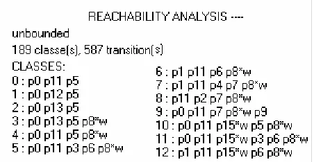
Our system is composed of 16 places and 15 transitions. Each transition possesses an interval of time (see Figure 4). The initial state of our net is e0 = (m0, D0) where m0 is the initial marking {p0, p11, p5} and D0 the interval associated with the transition t9 (0 ≤ t9 ≤ 1). t9 is initially the unique crossable transition; by its firing, the running process starts. Firing t9 since e0 at a date θ9 of [0.1] leads to the state e1 = (m1, D1) with m1: p0 p5 p12 and D1 the interval associated with the transition t10 (0 ≤ t10 ≤ 1). The firing of t10 leads us to the state e3 and so on (see Figure 4). The number of states can be very high if not infinite, which makes their handling much difficult. To solve this problem, we group states that have common characteristics in same classes [4]. One class includes all states made since the initial state by firing a single shot sequence. In our case, with TINA analysis shows that our system has 189 classes (see Figure 5).
Figure 5. Reachability analysis by TINA
III.3. Discussion of results
If one omits the time when modelling a real-time system [3], one can easily cause an unbounded net. Indeed, the consideration of these constraints slows the excessive time accumulation of tokens in specific places and forces the firing of certain transitions. The simulation of such a system based on time nets is closer to reality than non-time nets. Using TINA, we conclude that the system is not blocking and all the firings of transitions meet their time constraints. However, the system remains not bounded even with a finite number of states classes.
III. CONCLUSION
The aspects of competition, spontaneity, synchronization and others are well represented through these nets. Their extensions to cover specific needs, serve only to strengthen their widespread use. We used them to describe our system and to analyze it. The satisfaction of time constraints slows the rapid proliferation of the system states, reflected by the excessive accumulation of tokens in some places; however the system is still bounded.
To ensure that the system is bounded, we must enrich the existing constraints to retrieve a suitable scheduling. If the problem seems to be manageable in the case of one robot, it will not be the case with two robots and a single processor, and also in general for m robots and n processors. We plan to study these cases in our future work.
REFERENCES
[1] Alur R., Dill D.L., ‘’ A theory of timed automata ‘’, Theoretical computer science, vol. 126, n 2, 1994, p. 183-235.
[2] M. Andersen, R. Jensen, T. Bak and M. Quottrup,”Motion planning in multi-robot systems using timed automata”, 5th IFAC/EURON
[3] M.Azizi et M.Blej « Modélisation et Analyse d’un Système Robot à l’aide des Réseaux de Petri étendus », Maîtrise et Management des Risques industriels ENSA Oujda, Avril 2008
[4] B.Berthomieu and F.Vernadat Réseaux de Petri temporels:
méthode d’analyse et Vérification avec Tina.
http://dbserver.laas.fr/pls/LAAS/publis.rech_doc [5] B.Berthomieu and F.Vernadat,”Time Petri Nets Analysis
with TINA Symposium On Intelligent Autonomous Vehicles, July 2007.
http://dbserver.laas.fr/pls/LAAS/publis.rech_do
[6] Patrice Bonhomme: Réseaux de Petri p – temporels: contributions à la commande robuste. Thèse juillet 2001 – Université de Savoie
[7] F. Cassez et O.H.Roux: Traduction structurelle des Réseaux de Petri Temporels vers Les Automates Temporisé.
http://dbserver.laas.fr/pls/LAAS/publis.rech_doc
[8] A. Choquet-Geniet, G. Vidal-Naquet, « Réseaux de Petri et système Parallèles », Edition Armand Colin, 1993. [9] B. Damas and P. Lima,”Stochastic discrete event model of
a multi-robot team playing an adversarial game”, 5th IFAC/EURON Symposium On Intelligent Autonomous Vehicles, July 2004
[10]Diaz M, Senac P. « Time stream Petri nets: a model for timed multimedia information» Lecture Notes in Computer Science, vol. 815, 1994, p. 219
[11]A. Dominguez-Brito, M. Andersson and H. Christensen,”A software architecture for programming robotic systems based on the discrete event system paradigm”, Tech. Rep. CVAP244, ISRN KTH/NA/P-00/13-SE, September 2000. [12]B. Espiau, K. Kapellos, M. Jourdan and D. Simon,”On the
validation of robotics control systems part I: High level specification and formal verification”, Tech. Rep. 2719, February 1995.
[13]Emmanuel Grolleau, Annie Choquet-Geniet.
Ordonnancement de tâches temps réel en environnement multiprocesseur à l’aide de réseaux de Petri Real-Time Systems, RTS’2001, March 6-8 2001, Pari
[14]E. Grolleau and A. Choquet-Geniet, Off-line computation of real-time schedules by means of Petri nets, Workshop On Discrete Event Systems, WODES2000, Kluwer. Academic Publishers, Ghent, Belgium, pp. 309-316, 2000. [15]E. Grolleau and A. Choquet-Geniet, Scheduling real-time
systems by means of Petri nets, IFAC 25th Workshop on Real-Time Programming, WRTP'00, Palma de Mallorca, pp. 95-100, 2000
Rob´otica Instituto Superior T´ecnico Lisboa, Portugal {hcostelha,pal}@isr.ist.utl.p
[17]Khasa W, Denat J-P, Collart-Dutilleul S « P-Time Petri Nets for manufacturing systems », International Workshop on Discrete Event Systems, WODES'96, Edinburgh(U.K.), august 1996, p. 94.102
[18]J. Kosecka, H. Christensen and R. Bajcsy,”Experiments in behaviour composition”, Robotics and Autonomous Systems, vol. 19, pp. 287-298, March 1997.
[19] Merlin P.M, A study of the Recoverability of Computing systems, Irvine: Univ. California, These de doctorat, 1974. [20]Dejan Milutinovic; Pedro Lima: Petri Net Models of
Robotic Tasks. Proceedings of the 2002 IEEE International Conference on Robotics & Automation Washington, DC • May 2002
[21] Ramchandani C. ‘’ Analysis of asynchronous concurrent systems by timed Petri. nets’’, PhD thesis, Massachusetts Institute of Technology, Cambridge, MA, 1974, Project MAC Report MAC-TR -120
[22]Time Petri Net Analyser, http://www.laas.fr/tina, 2004
Mohammed Blej received his Master in analysis and computer science in 2004 from the Faculty of Sciences, Oujda, Morocco. He is currently a PhD student in the same faculty. His research interests include real time system, testing real time system, Petri nets, Task managing.
Mostafa azizi received his engineer diploma in Automatic and Industrial Computer Engineering in 1993 from the Mohammadia High School of Engineers (Rabat, Morocco). Then he received his Ph.D in Computer Science in 2001 from the University of
Montreal (Montreal, Canada). He is