Optimization-based Strategy for Polyomino Subarraying in Wideband Phased Array Design

(1)

International Doctorate School in Information and Communication Technologies

DISI - University of Trento

Optimization-based Strategy for

Polyomino Subarraying in Wideband

Phased Array Design

Roman Chirikov

Advisor:

Prof. Paolo Rocca

Universit`a degli Studi di Trento

Advisor:

Prof. Valeriy Bagmanov

Ufa State Aviation Technical University

(2)

(3)

First of all, I would like to thank Prof. Paolo Rocca and Prof. Andrea

Massa for inviting me to the Eledia group, teaching me and changing all

my life in the very best sense.

I thank Erasmus Mundus programme for financial support, in particular

Kerstin Kruse and Claudia Tarzariol.

I thank Silvano Gambadoro and Andrea Steccanella for the time we

worked together.

Special thanks go to Prof. Nafisa Yussupova for believing in me and

supporting me.

Many thanks to my teachers, colleagues and dear friends from USATU:

Prof. Albert Sultanov, Prof. Valeriy Bagmanov, Prof. Vladimir Vasiliev,

Prof. Vadim Kartak, Dr. Ivan Meshkov, Dr. Guzel Abdrakhmanova, Marat

Musakaev, Pavel Kucherbaev, Elizaveta Grakhova and others.

Thanks to my English teacher, Lidia Miniakhmetovna, for forcing me

to learn the language long before I ever needed it.

Finally, I thank my dearest Mama, Papa, Vova and Granddad for

(4)

(5)

Phased antenna arrays provide ultimate performance in areas where high directivity and electronic scanning are needed. That performance is achieved by involving large number of radiators as well as corresponding control units. As a result, such systems become bulky and heavy. In order to re-duce the number of control units, elements are grouped in subarrays with one of the control units, such as time delay, put at the subarray level. The drawback of this approach is that if elements are grouped into subarrays producing repetitive patterns in the array structure, radiation pattern of such array will be affected by undesired grating lobes. To eliminate that effect, subarrays of irregular shapes, such as polyominoes, are used. Still, those structures are an object for optimization. This work aims at apply-ing optimization techniques like genetic algorithm to the problem of findapply-ing optimal structures of phased antenna arrays composed of polyomino-shaped subarrays. For this purpose a new mathematical model, new algorithm and optimization methods are developed. Application of those techniques showed significant advances in radiation characteristics, in particular sidelobe level. Also new features were enabled, for example, multi-beam radiation pattern forming.

Keywords

(6)

(7)

1 Introduction and State-of-the-Art 1

1.1 Actuality of the problem of polyomino placement . . . 1

1.2 Analysis of existing methods and approaches to the

opti-mization of planar structures . . . 11

1.3 Goals and tasks of research . . . 18

1.4 Chapter 1 conclusions . . . 20

2 Development of mathematical model and optimization meth-ods for rectangular structures of polyominoes 21

2.1 Development of a mathematical model of antenna array

struc-tures built of polyomino-shaped subarrays . . . 21

2.2 Development of the optimization method based on the

struc-ture irregularity estimation . . . 29

2.2.1 Example values of irregularity by colour filtration

method . . . 35

2.2.2 Colour filtering method analysis . . . 38

2.3 Development of an optimization method based on

estima-tion of structure’s self-similarity . . . 41

2.3.1 Examples of self-similarity values by the

autocorre-lation method . . . 44

2.3.2 Autocorrelation method analysis . . . 47

(8)

3 Development of an optimization algorithm based on the

genetic algorithm 53

3.1 Problem of the genetic algorithm application . . . 53

3.1.1 Circular placement principle . . . 56

3.1.2 Fitness function . . . 59

3.1.3 Calibration of GA parameters . . . 62

3.1.4 Examples of structures by the Gwee—Lim algorithm 68 3.2 Development of the “Snowball” algorithm for optimization of structures of polyominoes . . . 74

3.2.1 Mathematical formulation . . . 75

3.2.2 Decoding strategy . . . 76

3.2.3 Fitness function . . . 80

3.2.4 Calibration of GA parameters . . . 81

3.2.5 Examples of structures by the “Snowball” algorithm 85 3.3 Comparison of the Gwee—Lim and “Snowball” algorithms by the fullness of structures . . . 91

3.4 Tiling with two shapes of polyominoes simultaneously . . . 94

3.4.1 Examples of structures by GLA with two shapes of polyominoes . . . 97

3.4.2 Examples of structures by SA with two shapes of polyominoes . . . 102

3.5 Comparison of the Gwee—Lim and “Snowball” algorithms by the fullness of structures with two shapes of polyominoes 107 3.6 Chapter 3 conclusions . . . 109

4 Application of the optimization algorithms to antenna ar-ray design 113 4.1 Applying Gwee—Lim algorithm to phased antenna array optimization . . . 114

(9)

by the sidelobe level . . . 125

4.4 Analysis of steering capabilities . . . 131

4.5 Analysis of bandwidth capabilities . . . 138

5 Multi-beam features of phased antenna arrays 149 5.1 Analysis of SLL for different angles between two beams . . 151

5.2 Application of the developed algorithm to two beams forming157 5.3 Chapter 5 conclusions . . . 171

6 Conclusions 173

Bibliography 175

(10)

(11)

1.1 Minimal estimation of number of different structures for

dif-ferent polyominoes . . . 10

2.1 Output data of the first example . . . 36

2.2 Output data of the second example . . . 37

2.3 Irregularity and SLL of structures of different sizes of

L-tromino . . . 38

2.4 Irregularity and SLL of structures of different sizes of

L-octomino . . . 39

2.7 Self-similarity and SLL of 32 × 32 structures of different

polyominoes . . . 48

2.8 Self-similarity and SLL of 64 × 64 structures of different

polyominoes . . . 48

2.9 Normalizing denominators ρ . . . 49

3.1 Average fitness function values at the first step of GLA

cal-ibration . . . 65

3.2 Average fitness function values of cubes at the first step of

GLA calibration . . . 66

3.3 Average values of the fitness function at the second step of

calibration of GLA . . . 68

(12)

3.6 Output data of the third example . . . 72

3.7 Output data of the fourth example . . . 73

3.8 Average fitness function values at the first step of SA cali-bration . . . 83

3.9 Average fitness function values of cubes at the first step of SA calibration . . . 84

3.10 Average values of the fitness function at the second step of calibration of SA . . . 86

3.15 Fullness of structures of different sizes by L-trominoes . . . 93

3.16 Fullness of structures of different sizes by L-octominoes . . 93

3.17 Fullness of a 32×32 structure with different polyominoes . 93 3.18 Output data of the first example . . . 98

3.26 Fullness of structures of different sizes with different pairs of polyominoes . . . 109

3.27 Fullness of a 32×32 structure with different pairs of poly-ominoes . . . 109

(13)

4.9 SLL of structures tiled with L-trominoes, ropt = 1.3 . . . . 126

4.10 SLL of structures tiled with L-trominoes, ropt = 1.818 . . . 127

4.11 SLL of structures tiled with L-octominoes, ropt = 1.3 . . . 128

4.12 SLL of structures tiled with L-octominoes, ropt = 1.818 . . 129

4.17 Output data of the fifth example . . . 136

4.18 Output data of the sixth example . . . 137

(14)

5.12 Output data of the seventh example . . . 165

5.13 Output data of the eighth example . . . 166

5.14 Output data of the ninth example . . . 167

5.15 Output data of the tenth example . . . 168

5.16 Output data of the eleventh example . . . 169

5.17 Output data of the twelfth example . . . 170

(15)

1.1 Example of a solution of an optimal packing problem . . . 3

1.2 Example of a radiation pattern in polar coordinates . . . . 5

1.3 Large phased antenna array for radio location . . . 6

1.4 Phased antenna array (a) and architecture of an element (b) 7 1.5 Radiation pattern of PAA with no subarraying in the sine

space . . . 8

1.6 PAA tiled with rectangular subarrays (a) and architecture

of subarrays (b) . . . 9 1.7 Picture of a PAA tiled with rectangular subarrays: front

view (a) and feeding network behind (b) . . . 10 1.8 Radiation pattern of a PAA built with rectangular subarrays 11

1.9 Polyomino shapes: L-shaped tromino (a), L-shaped tetro-mino (b), S-shaped tetromino (c), T-shaped tetromino (d), C-shaped octomino (e), L-shaped octomino (f), PU-shaped

octomino (g) . . . 12 1.10 Phased antenna array tiled with L-shaped octominoes . . . 13

1.11 Radiation pattern of PAA tiled with L-shaped octomino

subarrays . . . 14

1.12 Rectangular subarray placement on an irregular grid . . . 16

1.13 The “Danzer” structure . . . 16

1.14 The “Penrose” structure . . . 17

1.15 The “Sunflower” structure . . . 17

(16)

2.1 Element location in the structure . . . 23

2.2 Phase shift forming . . . 27

2.3 RGB model: three basic and three secondary colours . . . 31

2.4 Example of a structure in which polyominoes are painted in colours according to orientations . . . 32

2.5 Views of the structure in red (a), green (b) and blue (c) channels . . . 33

2.6 Array structure in the first example . . . 36

2.7 Array structure in the second example . . . 37

2.8 Irregularity and sidelobe level of structures of different sizes, tiled with L-trominoes . . . 38

2.9 Irregularity and sidelobe level of structures of different sizes, tiled with L-octominoes . . . 39

2.10 Irregularity and sidelobe level of structures of same size tiled with L-tromino . . . 40

2.11 Irregularity and sidelobe level of structures of same size tiled with L-octomino . . . 41

2.12 Serial scanning . . . 42

2.13 First six steps of the Hilbert curve . . . 43

2.14 Structure of an array in the first example . . . 45

2.15 Structure of an array in the second example . . . 46

2.16 Self-similarity and sidelobe level of 32 × 32 structures of different polyominoes . . . 47

2.17 Self-similarity and sidelobe level of 64 × 64 structures of different polyominoes . . . 49

2.18 Self-similarity and sidelobe level of structures of same size tiled with L-trominoes . . . 50

2.19 Self-similarity and sidelobe level of structures of same size tiled with L-octominoes . . . 51

(17)

3.4 Clarification of border edges and common edges [38] . . . . 60

3.5 Calibration space . . . 63

3.6 The first step of GLA calibration . . . 64

3.7 Second step of the GLA calibration . . . 67

3.8 Fitness function in the first example . . . 69

3.9 Fitness function in the second example . . . 69

3.10 Structure of the array in the first example . . . 70

3.11 Structure of the array in the second example . . . 71

3.12 Structure of the array in the third example . . . 72

3.13 Structure of the array in the fourth example . . . 73

3.14 Flowchart of the “Snowball” algorithm . . . 77

3.15 Orientations of L-shaped octomino with corresponding num-bers . . . 78

3.16 Search order of suitable positions . . . 79

3.17 Chromosome (3.17) decoding result . . . 80

3.18 The first step of SA calibration . . . 82

3.19 Second step of the SA calibration . . . 85

3.20 Fitness function in the fourth example . . . 86

3.21 Structure of the array in the first example without (a) and with margins (b) . . . 87

3.22 Structure of the array in the second example without (a) and with margins (b) . . . 88

3.23 Structure of the array in the third example without (a) and with margins (b) . . . 89

3.24 Structure of the array in the fourth example without (a) and with margins (b) . . . 90

(18)

3.25 Fullness of structures of different sizes by L-trominoes . . . 92

3.26 Fullness of structures of different sizes by L-octominoes . . 94

3.27 Fullness of a 32×32 structure with different polyominoes . 95 3.28 A 32×32 structure, tiled by GLA with C-octominoes . . . 95

3.29 A 32×32 structure, tiled by SA with C-octominoes . . . . 96

3.30 Extended genes in a chromosome . . . 96

3.32 Array structure in the first example . . . 98

3.33 Array structure in the second example . . . 99

3.34 Array structure in the third example . . . 100

3.35 Array structure in the fourth example . . . 101

3.37 Array structure in the first example without (a) and with (b) margins . . . 103

3.38 Array structure in the second example without (a) and with (b) margins . . . 104

3.39 Array structure in the third example without (a) and with (b) margins . . . 105

3.40 Array structure in the fourth example without (a) and with (b) margins . . . 106

3.41 Fullness of structures of different sizes by L-trominoes and L-octominoes . . . 108

3.42 Fullness of structures of different sizes by L-tetrominoes and L-octominoes . . . 110

3.43 Fullness of a 32×32 structure with different pairs of poly-ominoes . . . 111

4.1 Structure of the software . . . 114

(19)

4.6 Radiation pattern in the fourth example at r = 1.3 . . . . 119

4.8 Radiation pattern in the first example at r = 1.3 . . . 121

4.9 Radiation pattern in the second example at r = 1.3 . . . . 122

4.10 Radiation pattern in the third example at r = 1.3 . . . 123

4.12 SLL of structures tiled with L-trominoes, ropt = 1.3 . . . . 126

4.13 SLL of structures tiled with L-trominoes, ropt = 1.818 . . . 127

4.14 SLL of structures tiled with L-octominoes, ropt = 1.3 . . . 128

4.15 SLL of structures tiled with L-octominoes, ropt = 1.818 . . 129

4.16 SLL comparison for structures of different sizes of L-octominoes,

obtained by GLA, SA and R. Mailloux [59] . . . 130

4.22 Radiation pattern in the fifth example at r = 1.3 . . . 136

4.23 Radiation pattern in the sixth example at r = 1.3 . . . 137

4.24 SLL at different steering angles . . . 138

4.25 Radiation pattern in the first example at r = 1.333 . . . . 139

4.26 Radiation pattern in the second example at r = 1.500 . . . 140

4.27 Radiation pattern in the third example at r = 1.600 . . . . 141

4.28 Radiation pattern in the fourth example at r = 1.667 . . . 142

4.29 Radiation pattern in the fifth example at r = 1.750 . . . . 143

4.30 Radiation pattern in the sixth example at r = 1.818 . . . . 144

(20)

4.33 SLL at different bandwidths . . . 147

5.1 Structure of the array in the first example . . . 150

5.2 Radiation pattern for structure in figure 5.1 at r = 1.3 . . 150

5.4 Radiation pattern in the first example at r = 1.300 . . . . 152

5.5 Radiation pattern in the second example at r = 1.300 . . . 153

5.6 Radiation pattern in the third example at r = 1.300 . . . . 154

5.7 Radiation pattern in the fourth example at r = 1.300 . . . 155

5.9 SLL and beam power difference for various angles . . . 157

5.10 Fitness function in the fourth example . . . 158

5.17 Radiation pattern in the seventh example at r = 1.3 . . . . 165

5.18 Radiation pattern in the eighth example at r = 1.3 . . . . 166

5.19 Radiation pattern in the ninth example at r = 1.3 . . . 167

5.20 Radiation pattern in the tenth example at r = 1.3 . . . 168

5.21 Radiation pattern in the eleventh example at r = 1.818 . . 169

5.22 Radiation pattern in the twelfth example at r = 1.818 . . . 170

(21)

The thesis consists of chapters as follows.

The first chapter contains analysis of the field of phased antenna arrays

together with the state-of-the-art. The actual problem is formulated. Also

the topic of optimization is discussed on examples of several common tasks

and various techniques are listed.

The second chapter describes development of the mathematical model

of planar phased antenna arrays built of polyomino-shaped subarrays. Two

optimization methods based on that model are also developed and

anal-ysed.

Chapter 3 describes the problem of application of the genetic algorithm

and shows in details the algorithm for polyomino placement by Gwee and

Lim. Then the “Snowball” algorithm is developed and compared to the

Gwee—Lim algorithm with examples.

Chapter 4 is dedicated to the analysis of antenna array structures

ob-tained by two algorithms. It shows advantages of the developed algorithm

in terms of sidelobe level suppression.

Chapter 5 includes several examples and analysis of multi-beam

radia-tion patterns obtained by structures with two shapes of subarrays. They

show further enhancements of the array technology.

(22)

(23)

Introduction and State-of-the-Art

1.1

Actuality of the problem of polyomino placement

The task of optimization of technological processes and solutions has always

been a part of a technical thinking. Optimization is a process of finding an

optimal solution. Optimal solution is the one that is more preferable than

other according to some criteria [86].

Optimization of technological processes can be divided into four general

groups.

• Time optimization means that the process should run as fast as pos-sible. For example, the slowest part of a conveyor may need to be

optimised to increase productivity of the whole assembly process.

• Raw materials optimization pursues the most effective usage of the needed raw materials. As an example one may consider optimization

of a shape of a plastic cover of some unit to decrease the consumption

of plastic [42].

• Cost optimization in opposite of raw materials optimization supposes minimization of all the costs including salary and equipment.

• Quality optimization has a goal of reaching the best quality in a

(24)

1.1. ACTUALITY OF THE PROBLEM OF POLYOMINO PLACEMENT

cess. The example is manual potato cleaning instead of automated.

The process becomes expensive and long but the quality increases.

In a similar way optimization of technological solutions is made in

ac-cordance with some set of criteria. The set may consist of one or more

criteria. Under a technological solution may be considered a solution of

some problem by applying an existing technology as well as some system in

a broad sense. Optimization of a system may be focused on choosing the

optimal components of the system, optimization of connections (including

spatial) between them or all together.

Optimal placement of a set of objects in a limited space represents a wide

class of optimization problems. Usually such space is a rectangular area

on a plane while objects are geometrical shapes, real objects or even

ab-stract objects represented in geometrical shapes.Further examples of such

problems are listed. All of them belong to NP-hard class of problems.

Optimal packing problem. This problem is classical in such areas as system analysis, combinatorics and linear algebra. This problem can be

formulated like: there is a container of a given shape in which the maximum

number of objects again of given shapes should be placed. The objects may

be of different shapes and sizes. Such a problem has been investigated in a

one-dimensional [35], two-dimensional [80, 12], three-dimensional [87] and

multidimensional variations. In figure 1.1 an example of a solution of such

problem is shown.

Optimal cutting problem. The difference of this problem is that there are several shapes into which a sheet of some material should be cut.

The point is to minimize the garbage from cutting, i.e. maximization of

the density of the shape placement. This problem is studied in several

well-known works [30, 29, 46].

The rucksack problem. This problem is different from the previous ones because it is multi-criterial by definition. The essence is in the

(25)

Figure 1.1: Example of a solution of an optimal packing problem

lowing: there is a rucksack of a limited volume. There is a set of objects

of given sizes and prices. It is needed to put in the rucksack such a set of

objects so that their total cost would be maximal. There is a variation of

this problem where instead of the limit of the volume there is a limitation

of its load capacity and the objects have weight instead of price.

But along with the listed above problems there is an important task of

optimization of the structures of phased antenna arrays built with irregular

subarrays in order to increase their energy efficiency, communication range

and electromagnetic interoperability. The topic of this work is in the area

of optimization of a system that consists of a fuzzy set of components

with particular properties and two types of connections — geometrical

and electrodynamic. Both connections will be studied during the process

of the mathematical model development.

First of all it is necessary to explain what is a phased antenna array

and what is it used for. An antenna is a device for radiating or receiving

electromagnetic waves. Antennas are the key elements in such well-known

areas as wireless communication, radio location and radio astronomy. In

recent years the research in wireless energy transfer has got an impulse.

Antennas can be of various types, shapes and sizes. But there are several

basic parameters applicable for all of them:

(26)

1.1. ACTUALITY OF THE PROBLEM OF POLYOMINO PLACEMENT

• radiation pattern (RP) — graphical representation of dependence of gain or directivity of the antenna on the direction in a given plane;

• gain — ratio of input power of the reference antenna to the input power of the given antenna given that both antennas produce the

same electric field intensity in one direction at the same distance or

same power flux density;

• directivity — ratio of squared electric field intensity produced by the antenna in a given direction to the average square of electric field

intensity in all directions;

• sidelobe level (SLL) — relative (normalized to the maximum of RP) level of antenna radiation in direction of side lobes;

• front-to-back ratio (F/B) — ratio of the front radiation level to the back radiation level;

• beamwidth — angle within which the radiation level is higher than half of the level of the main beam (or in other words, less than the

maximum for 3 dB or less).

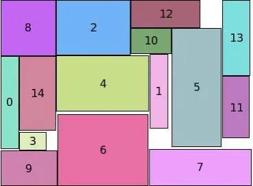
In figure 1.2 a typical radiation pattern is shown in polar coordinates.

It has a main beam and side lobes including a backside lobe.

In some cases there are special requirements for the antenna parameters,

such as high gain or ability to change radiation pattern. In such cases

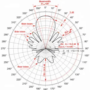
phased antenna arrays (PAA) are used (figure 1.3). Antenna arrays are

complex systems consisting of two or more equal antennas joined by one

feeding network and functioning in coherence. Radiators belong to passive

components. Phased arrays differ by having active components such as

amplifiers and phase shifters. PAAs have the ability to apply amplitude and

phase corrections at every radiator (array element) forming therefore the

(27)

Figure 1.2: Example of a radiation pattern in polar coordinates

needed radiation pattern. Sharp RP increases the quality of transmitting

and receiving signals in a given direction decreasing the noise level coming

from other directions. PAA may be linear, when all elements are aligned

in one line, and planar, when elements lie in a plane.

In order to increase the throughput of wireless communication systems

in recent years a shift towards wideband systems has been initiated [81, 43].

The feature of those systems is wide signal spectrum, i.e. a big set of

frequencies of electromagnetic waves is used for signal transmission [77].

As it was said, PAA can change its radiation pattern, i.e. steer its main

beam [71]. In case of wideband systems and/or large antenna array the

phase shifters cannot handle the task of beam forming [49]. In this case

time delay (TD) is required. Such arrays find their application in radio

(28)

1.1. ACTUALITY OF THE PROBLEM OF POLYOMINO PLACEMENT

Figure 1.3: Large phased antenna array for radio location

location, radio astronomy and communication systems [32].

A PAA of 8 × 8 elements is shown in figure 1.4a. Every element has the same architecture behind it shown in figure 1.4b. A typical radiation pattern is presented in figure 1.5. The RP is shown in three-dimensional

sine space (discussed in more details in chapter 3). The radiation level

is expressed in decibels relatively to the main beam. The simulation was

run with the beam steering to angle (45◦; 45◦) that corresponds to sine

space coordinates (0,5; 0,5). As it is seen from RP, there is one strongly

pronounced beam and two rows of weak side lobes in accordance with

Taylor current distribution [82].

The problem of time delay components is that they are significantly

more expensive, bigger and heavier than other components. If we don’t

consider the cost, their application is still limited in satellite

communica-tions due to its weight. To solve this problem by sacrificing the performance

(29)

Element (a)

Radiator

Amplifier

Phase shifter

τ

Time delay

(b)

Figure 1.4: Phased antenna array (a) and architecture of an element (b)

it was proposed to split PAA into subarrays and put one time delay

com-ponent before subarray input, i.e. move time delays to the subarray level

[79, 78]. Therefore, the number of needed time delays decreases

propor-tionally to the number of elements grouped in one subarray. In figure 1.6

a 8×8 PAA is shown tiled with subarrays of 4×2 elements.

There is another problem with subarrays. The delay of a signal formed

by the time delay is true only for that point of an array that it was

cal-culated for. Let us consider that TD is placed under the central element

of a subarray and the value of the delay is calculated for that element. In

this case an error will be generated on all other elements of the subarray

represented by a time shift of the signal. To be exact, it should be

re-minded that this effect occurs only for wideband systems. Every element

receives its own error value and own time shift. That shift is the same

for corresponding elements of neighbour subarrays. Consequently, the

(30)

1.1. ACTUALITY OF THE PROBLEM OF POLYOMINO PLACEMENT -1 -0.5 0 0.5 1 -1 -0.5 0 0.5 1 -60 -50 -40 -30 -20 -10 0 Radiation, dB u v Radiation, dB -60 -50 -40 -30 -20 -10 0

Figure 1.5: Radiation pattern of PAA with no subarraying in the sine space

nal from those elements is coherently added and amplified. It turns out

to be an error accumulation. This error is represented in grating lobes

in the RP that happen to be side lobes [68]. Their existence is highly

undesired because they lead to decrease in power of the main beam and

affect the electromagnetic interoperability of a system. Note that the error

accumulation from the corresponding elements happens due to the regular

placement of subarrays in the array. The illustrative radiation pattern is

shown in figure 1.8. Besides the main beam it has five strong side lobes

with the highest level at −9,5 dB.

One of the ways to overcome the occurrence of strong side lobes is to

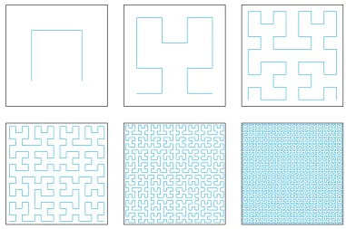
use the subarrays of irregular shape, namely polyomino-shaped (figure 1.9)

[56]. Character C defines the centre. Such shapes rotated by a multiple

of 90 degrees allow to eliminate the regularity in the subarray placement

and, therefore, prevent the error accumulation. Figure 1.10 shows the same

8×8 structure tiled this time with L-shaped octominoes. On the radiation

(31)

(a)

τ

Radiator

Phase shifter Amplifier

Time delay

(b)

Figure 1.6: PAA tiled with rectangular subarrays (a) and architecture of subarrays (b)

pattern (figure 1.11) it can be seen that the side lobes are spread over the

whole space, decreasing therefore its maximum down to −20,3 dB.

PAA of the same size in one and the same frequency band but with

different structures, obviously, produce different level of side lobes. It is

easy to estimate the minimal number of possible structures of size M ×N

elements tiled with polyomino with q cells. Let us define the area of a

(32)

1.1. ACTUALITY OF THE PROBLEM OF POLYOMINO PLACEMENT

(a) (b)

Figure 1.7: Picture of a PAA tiled with rectangular subarrays: front view (a) and feeding network behind (b)

minimal rectangle completely tiled with such a polyomino as Smin. Inside

this rectangle Smin/_q polyominoes are placed unambiguously. This rectangle

can be rotated by 90 degrees or flipped. In total there are four possible

minimal rectangles. Inside the structure there can be M ×N_/_S

min such

rect-angles. So, we can say that the minimal number of various structures with

full coverage is

NK =

2Smin

q

M_S×N

min

. (1.1)

In table 1.1 this number has been calculated for some polyomino types.

As it is seen, even the minimal estimation of the structures number prevents

from using brute force search for the optimal structure larger than 8 ×8

according to some criteria. Therefore, an approximate method is needed.

Table 1.1: Minimal estimation of number of different structures for different polyominoes L-tromino L-tetromino L-octomino

8×8 2642246 6536 256 16×16 4.87·1025 ₁_.₈₄_·₁₀19 ₄_.₂₉_·₁₀9

32×32 5.64·10102 1.16·1077 3.4·1038

In papers by Mailloux [59, 61] such structures were composed manually

(33)

-1

-0.5

0

0.5

1 -1

-0.5 0

0.5 1 -60

-50 -40 -30 -20 -10 0

Radiation,

dB

u

v

Radiation,

dB

-60 -50 -40 -30 -20

Figure 1.8: Radiation pattern of a PAA built with rectangular subarrays

without any optimization. The question of choosing particular structure

was not stated. So, there is an actual problem of optimization of phased

antenna arrays structures tiled with polyomino-shaped subarrays.

Therefore, the actuality of the problem was shown. Practical

applica-tion field was described in details, in which phased antenna arrays act as

complex spatially distributed objects. Problems were shown that occur in

design of large phased antenna arrays with polyomino-shaped subarraying.

1.2

Analysis of existing methods and approaches to

the optimization of planar structures

In the previous section the urgency of the research topic was described.

Now it is necessary to analyse the state of the art. Analysis of the

achieve-ments in the field will be performed from two sides. From one side, methods

and algorithms for optimization of two-dimensional structures, tiled with

(34)

1.2. ANALYSIS OF EXISTING METHODS AND APPROACHES TO THE OPTIMIZATION OF PLANAR STRUCTURES

C C C

C

C C C

a b c d

e f g

Figure 1.9: Polyomino shapes: L-shaped tromino (a), L-shaped tetromino (b), S-shaped tetromino (c), T-shaped tetromino (d), C-shaped octomino (e), L-shaped octomino (f), PU-shaped octomino (g)

objects of irregular shape, would be considered. That is geometric or

sys-tem component of the work will be analysed. From the other side, the

analysis of sidelobe level suppression methods in phased antenna arrays

will be performed.

There are analytical and empirical methods of packing objects in

struc-tures. For example, Chinn and Grimaldi in their work analytically pack

polyominoes into rectangular areas of the smallest size, which then cover

the structure [14].

Opting empirical methods was done for the following reasons:

1. Such evaluation criterion of a PAR structure as the sidelobe level is in

the complex implicit dependence on the structure itself and can only

be calculated by modelling the entire system. Thus, the optimization

problem is finding the global maximum in the large discrete space of

solutions [85].

2. number of structures that can be obtained by filling a large rectangular

(35)

Figure 1.10: Phased antenna array tiled with L-shaped octominoes

area with polyominoes is so big that it is not possible to sort out all

the options and model them.

Empirical methods include optimization, that implements search for

so-lutions in some complex multidimensional space. There are a number of

studies that have compared different optimization algorithms such as

parti-cle swarm optimization method with genetic algorithm [40, 31],

evolution-ary algorithms [4, 63] and ant colony optimization [73]. Some researchers

are interested in combining particle swarm optimization with such genetic

mechanisms as breeding and selection [55, 5, 65]. Many variations of the

original method of particle swarm optimization were suggested. For

ex-ample, parallel optimization of several smaller swarms [83, 75, 84], adding

negative entropy for mixing the particles [91], dissemination of findings

within a limited number of nearest neighbours [48, 50, 62, 47], variation of

searching objects in time [3], application of the particle swarm optimization

method for controlling mutation in the evolutionary methods [89],

disper-sal of clustered particles to increase diversity [54], application of fuzzy logic

(36)

1.2. ANALYSIS OF EXISTING METHODS AND APPROACHES TO THE OPTIMIZATION OF PLANAR STRUCTURES

-1 -0.5 0 0.5 1 -1 -0.5 0 0.5 1 -60 -50 -40 -30 -20 -10 0 Radiation, dB u v Radiation, dB -60 -50 -40 -30 -20 -10 0

Figure 1.11: Radiation pattern of PAA tiled with L-shaped octomino subarrays

for adjusting the parameters of the algorithm [74]. Daniel Boeringer and

Douglas Werner compared particle swarm optimization with the genetic

algorithm [8] and showed that the latter has a better ability to beam

form-ing. There are examples of the use of genetic algorithm in electromagnetics

and antenna design [90, 2].

Among the empirical methods we have chosen the genetic algorithm

(GA) for the following reasons:

1. Independence from the task type. In this work the task is a battery

of many parameters for which the optimal value has to be found.

2. Discreteness of the nature of the task. Since PAAs have regular grid

and polyominoes are placed in the nodes of that grid with strictly

defined possible orientations, the search space is discrete.

3. Continuous actual range of the cost function. In opposite to the search

space, the criteria that describe potential solutions are continuous

(37)

Now let us face the question of sidelobe level suppression. As it was

mentioned, grating lobes appear due to the accumulation of the phase shift

error among regularly placed subarrays. The subarrays and elements inside

them could be placed within a periodic and an aperiodic grid. In the first

case the array is called equidistant and in the second — non-equidistant.

The shape of the subarrays can be rectangular and irregular. Accordingly,

there are four domains of planar array subarraying.

The first domain represents the simplest case, when rectangular

subar-rays are put into a periodic grid. In other words, the array is being split

into equal rectangle areas of several radiating elements. Although in this

case the area of the array is simply and effectively filled (figure 1.6), the

corresponding radiation pattern is characterized by poor radiation

perfor-mance with grating lobes due to the periodicity of the structure (figure 1.8)

[60].

Other three domains aim at breaking this periodicity in different ways.

In the second domain the rectangular subarrays are arranged in an

ape-riodic grid, which results in small arbitrary relative displacements and/or

rotations (figure 1.12) [51]. This is the simplest solution for breaking

pe-riodicity. This solution is still simple from the point of view of production

process but the achieved sidelobe suppression is not high (around 11 dB)

[52].

The third domain is represented by irregular subarrays that

aperiodi-cally tile the aperture of the array [76, 88]. Here subarrays of more than

one irregular shape are used simultaneously and placed in an aperiodic

order, thus in nodes of an irregular grid.

One of the examples is the “Danzer” structure by Thomas Spence and

Douglas Werner [76]. Their structure consists of many various triangles

each being a subarray (figure 1.13). Such an array produces sidelobes of

(38)

1.2. ANALYSIS OF EXISTING METHODS AND APPROACHES TO THE OPTIMIZATION OF PLANAR STRUCTURES

Figure 1.12: Rectangular subarray placement on an irregular grid

−17.3 dB.

Figure 1.13: The “Danzer” structure

Pierro with colleagues published a structure called “Penrose” [66]

(fig-ure 1.14). It also contains a lot of subarrays and suppresses SLL down to −17 dB.

A very beautiful variant of an antenna array structure was shown by

Vigan´o [88]. It is called “Sunflower” (figure 1.15) and also keeps SLL at

level of −17 dB.

(39)

called “Pinwheel” [69]. In their article Morabito and others declare SLL

suppression to −21.5 dB.

Figure 1.14: The “Penrose” structure

Figure 1.15: The “Sunflower” structure

(40)

1.3. GOALS AND TASKS OF RESEARCH

The results achieved in this domain are significant due to high

irregular-ity of the array structures (also considering arbitrary placement of elements

within a subarray) [64, 66]. Although, the structures become very complex

and include a big number of elements, which leads to high costs of the

arrays and their size and weight.

Accordingly, the fourth domain — the use of subarrays of irregular

shapes placed onto a periodic grid — has been adopted to avoid the

pres-ence of grating lobes of the array factor [57]. This approach provides good

sidelobe level suppression still keeping the structure feasible in terms of

mass production (figure 1.11). Having one irregular shape of a subarray

it is possible to produce them first and then use them to build the whole

array, just rotating the shape. Circular polarization used in

communica-tion systems will not be ruined. The quescommunica-tion that arises is how to obtain

such a structure to meet particular requirements. In other words, the array

structure has to be optimized. The problem of large array tiling with

sub-arrays of irregular shape comes to finding subarray positions with minimal

number of holes (i.e. uncovered cells), that decrease the gain, and avoiding

periodicity in subarray placement in order to minimize the number and

level of the side lobes [6].

Therefore, existing methods and approaches to the problem of

opti-mization of planar structures were analysed. Separately the optiopti-mization

methods for phased antenna array structures were considered.

Disadvan-tages of those methods applied to antenna array design were indicated and

the way of research was chosen.

1.3

Goals and tasks of research

After substantiating actuality and analysing present methods and

appro-aches, the goal of the work was set to be an increase of operating efficiency

(41)

optimization of their structures composed of polyomino-shaped subarrays.

The choice of the genetic algorithm is grounded on the features of the

application field. Phased antenna array optimization is one of the ways

to fulfil the growing requirements for wireless communication speed and

electromagnetic interoperability. The following research tasks have been

formulated:

1. To develop a mathematical model of a phased antenna array structure

composed of polyomino-shaped subarrays. This model should join

geometric properties of the system, common for all planar structures,

and electrodynamic properties that are specific for antenna arrays.

The development of the model lies in the base of the whole research

and is a fundamental step for further activities.

2. To develop a optimization method for polyomino placement based on

a criterion of estimation of irregularity of structures. The sidelobe

level of an antenna array that is being optimized is connected with

subarray placement in the structure, more exactly with their

irreg-ularity. Therefore, by the irregularity estimation of a structure it is

possible to estimate the sidelobe level. This task plays an important

role in universalization of the algorithm to be developed.

3. To develop an algorithm of a structural-parametric synthesis of

struc-tures of polyominoes. This is the main theoretical task of the work.

The algorithm is meant to synthesize structures, optimized by given

criteria applying developed methods.

4. To develop a software based on the proposed algorithm for solving the

phased antenna array optimization problem. The task has both

theo-retical — parameters calibration — and practical sides — synthesis of

(42)

1.4. CHAPTER 1 CONCLUSIONS

antenna array structures. The software is needed for testing the

algo-rithm and running numerical simulations on the obtained structures.

5. To assess the efficiency of the proposed algorithm and obtained

struc-tures by the mathematical simulation. Using the software it is needed

to get output results of the algorithm and to analyse them, proving

that the goal is achieved.

1.4

Chapter 1 conclusions

1. The actuality of the problem was shown. Practical application field

was described in details, in which phased antenna arrays act as

com-plex spatially distributed objects. Problems were shown that occur in

design of large phased antenna arrays with polyomino-shaped

subar-raying.

2. Existing methods and approaches to the problem of optimization of

planar structures were analysed. Separately the optimization methods

for phased antenna array structures were considered. Disadvantages

of those methods applied to antenna array design were indicated and

the way of research was chosen.

3. The goal of the work was formulated according to analysis of the state

of the art in the field. The scientific tasks were stated that will lead

to the goal achievement by a consistent progress.

(43)

Development of mathematical model

and optimization methods for

rectangular structures of

polyominoes

2.1

Development of a mathematical model of antenna

array structures built of polyomino-shaped

sub-arrays

First of all in order to solve the optimization problem it is necessary to

formulate and describe it mathematically. Moreover, except for the static

characteristics of the whole system it is required to describe the relations

between the system components, as well as the characteristics of the

com-ponents. This is called the development of a model of the system. The

model reflects all the necessary properties of the system and its

compo-nents and its response to external stimuli. Only having a correct model of

the system one can develop methods and algorithms for optimization and

be sure they are adequate. Main results of the chapter are published by

the author in journals and conference proceedings [16, 18, 21, 70, 23].

(44)

2.1. DEVELOPMENT OF A MATHEMATICAL MODEL OF ANTENNA ARRAY STRUCTURES BUILT OF POLYOMINO-SHAPED SUBARRAYS

Thus, the model of the same system may be different for different

appli-cations. For example, for the calculation of the deformation forces of the

bridge, a model is needed that takes into account the type, size and

mate-rial of the structure. If we need a model for visualizing the same bridge, it

will contain information about the shape, size and colour of the bridge.

The theme of this work is to optimize rectangular structures on the

example of antenna arrays. Accordingly, it is necessary at first to consider

the characteristics of the antenna arrays and to decide which criteria will be

used in the optimization of the characteristics and which must be present

in the model. Thereafter, these features must be combined into a single

mathematical apparatus capable in terms of the laws of physics to reliably

describe the antenna array.

In the first chapter it was mentioned that the antenna array is a

sys-tem in which there are two types of inter-element relations: geometric and

electromagnetic. Also there was a list with definitions of the main

char-acteristics of antennas: radiation pattern, gain, directivity, sidelobe level,

front-to-back ratio, beamwidth.

The usage of subarrays of different polyomino shapes (figure 1.9) in the

design of the antenna array was originally aimed at the suppression of

side lobes in the radiation pattern. However, the maximum suppression

of SLL does not mean the maximum coverage of the array by subarrays.

If a portion of the array is not included into any subarray, this means

that in this area (which may consist of one or more elements) no radiating

elements are set. Such areas are called holes. Large number of holes in the

array reduces the antenna gain, which affects both the receiving and the

transmission of signal. Thus, the optimization criteria selected are sidelobe

level and geometric fullness of the array.

In this work planar rectangular equidistant antenna arrays are

consid-ered. They are rectangular planar structures consisting of equal-sized cells.

(45)

have M rows and N columns and lies in the x−y plane, where rows are

parallel to the axis x, and the columns to axis y (Figure 2.1).

dx

dy

x

y

1 2 3 N

1

2

3

M 0

Figure 2.1: Element location in the structure

As was already mentioned, the antenna arrays consist of identical

emit-ters. The distance between the centers of the elements in an equidistant

array are the same too within the axes. Note that the physical

dimen-sions of the radiators do not play an important role in the work and are

not counted. It is supposed that the dimensions of the emitters are small

enough to fit in a predetermined inter-element distance, which is set in the

wavelengths at the central frequency of the bandwidth. Accordingly, we

denote the inter-element distance along the axes x and y as dx and dy.

An empty structure is represented by a zero-filled matrix [45]:

A =

     

0 0 · · · 0

0 0 · · · 0 ... ... ... ... 0 0 · · · 0

     

(2.1)

As filling the structure with polyomino forms, matrix elements belonging

to those polyominoes are assigned sequence numbers, starting with one.

(46)

2.1. DEVELOPMENT OF A MATHEMATICAL MODEL OF ANTENNA ARRAY STRUCTURES BUILT OF POLYOMINO-SHAPED SUBARRAYS

Each shape of polyomino may be rotated inside the structure by an angle

that is a multiple of 90 degrees. In addition, the polyomino can be flipped

that adds four more orientations. In total there are eight orientations.

Each of the orientations may be provided by a separate matrix with two

columns and as many rows as the number of elements in polyomino without

one. Matrix elements are the coordinates defining the location of each

element relative to a pre-determined center of the polyomino. Each row of

this matrix determines the shift of each element polyomino (except center)

relative to the center. The first column specifies the offset for axis y,

and the second for axis x. For example, the L-shaped octomino comprises

eight elements. To describe its orientations we need to make eight matrices

of 7 × 2 elements. Following are the eight orientations of L-octomino in

accordance with figures 1.9 and 3.15:

T0 =

             −2 −1 −1 −1 0 −1 0 1 1 −1 1 0 1 1             

, T1 =

             −1 −1 −1 0 −1 1 −1 2 0 −1 1 −1 1 0             

, T2 =

             −1 −1 −1 0 −1 1 0 −1 0 1 1 1 2 1              ,

T3 =

             −1 0 −1 1 0 1 1 −2 1 −1 1 0 1 1             

, T4 =

             −2 1 −1 1 0 −1 0 1 1 −1 1 0 1 1             

, T5 =

(47)

T6 =              −1 −1 −1 0 −1 1 0 −1 0 1 1 −1 2 −1             

, T7 =

             −1 −2 −1 −1 −1 0 −1 1 0 1 1 0 1 1              .

These matrices are used by the program and stored in separate files.

Possessing a structure matrix and polyomino orientations matrix, we can

formulate the condition of possibility of polyominoes placement (in our

example, L-octomino) at position (x, y). It is understood that the center

of polyomino is located at coordinates (x, y) and the other elements —

according to their relative shifts identified by vectors in an orientation

matrix. Subarrays can not be superimposed on each other, respectively a

polyomino can not be put in the structure, if at least one element of it is in

already occupied place. It is easy to figure it out. It is enough to compute

the sum of elements of the structure matrix, found in the coordinates from

the orientation matrix. Here also a ban is included on crossing border

of the structure — all polyominoes must be located entirely within the

structure:

Yµ(x, y) =

    

Ax,y + q−1

P

i=1

Ax1,y1, 06 x1 < N ∧06 y1 < M;

1, x1 < 0∨x1 > N ∨y1 < 0∨y1 >M;

(2.3)

x1 = x+T_i,µ₂, y1 = y +T

µ i,1,

whereµ— orientation of polyomino,q — number of elements in polyomino.

If Y = 0 then the placement of the polyomino at a given location is

(48)

2.1. DEVELOPMENT OF A MATHEMATICAL MODEL OF ANTENNA ARRAY STRUCTURES BUILT OF POLYOMINO-SHAPED SUBARRAYS

an example of placement of the first L-octomino with orientation number

zero (matrix T0) into an empty structure of size 8×8 at the center with

coordinates (4,4):

A =                

0 0 0 0 0 0 0 0

0 0 1 0 0 0 0 0

0 0 1 1 1 0 0 0

0 0 0 0 0 0 0 0

                (2.4)

Therefore, we have a model of a structure (array matrix), model of

poly-ominoes (orientation matrices) and conditions for polyomino placement.

This set lets us to describe and consider geometric relations between the

elements in a system.

As well as geometric, we need to consider electrodynamic relations to

compute the radiation pattern. It is well known that the far field of an

antenna array E(θ, φ) is derived from the field of a single element:

E(θ, φ) = E1(θ, φ)×AF(θ, φ), (2.5)

where θ and φ — spherical coordinates, E1 — single element field, AF —

array factor. For ease, instead of spherical coordinates they use sine space

coordinates [67]:

u = sinθcosφ,

v = sinθsinφ. (2.6)

The array factor characterizes the interference of radiation from single

(49)

The standard notation is the following:

AF(θ, φ) =

M

X

m=1

N

X

n=1

amne−jk[mdx(u−u0)+ndy(v−v0)], (2.7)

where amn — amplitude coefficient that sets amplitude distribution, k =

2π_/_λ _{— wave number,} _λ _{— wave length,} _u0 _and _v0 _{— steering angle of}

the main beam. The exponent defines the phase shift from phase shifter.

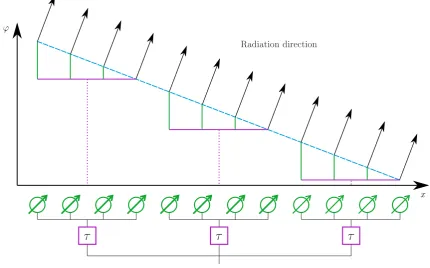
Figure 2.2 shows a simplified scheme of phase shift forming in a linear

antenna array composed of three subarrays with four elements in each. The

y axis measures the signal phase of each element. Linear phase distribution

through the array provides the forming of the main beam in the desired

direction.

x ϕ

τ τ τ

Radiation direction

Figure 2.2: Phase shift forming

Equation (2.7) supposes that beneath each element in the array there is

(50)

2.1. DEVELOPMENT OF A MATHEMATICAL MODEL OF ANTENNA ARRAY STRUCTURES BUILT OF POLYOMINO-SHAPED SUBARRAYS

Let the array of size M×N be completely filled with rectangular subarrays

of size M0 × N0 (figure 1.6a) with architecture according to figure 1.6b.

Subarray factor will be written as:

SAF(θ, φ) =

M0 X m=1 N0 X n=1

amne−jk[mdx(u−u0)+ndy(v−v0)]. (2.8)

Array factor will be expressed through subarrays as:

AF(θ, φ) = M_/_M

0

X

m0=1

N_/_N

0

X

n0=1

SAF(θ, φ)e−j2πf τm₀n₀_, _(2.9) where f — frequency, τ — time delay value from the time delay element,

that can be calculated for rectangular subarrays placed regularly:

τm0n0 =

1

c [cm + (m0 −1)M0dx] (u−u0) +

1

c [cn+ (n0 −1)N0dy] (v−v0),

(2.10)

where c — speed of light and cm and cn — subarray center coordinates

relatively to top left corner.

In case of polyomino-shaped subarrays the situation becomes more

com-plicated, because polyominoes and their centres are located not regularly.

Actually, for this they are used. However, they can also be described

math-ematically, meaning that we know all the orientations matrices and centre

coordinates for each of them. Subarray factor will be expressed as:

SAF(θ, φ) =

q−1

X

i=1

aie−jk[T

µ

i,2dx(u−u0)+Ti,µ1dy(v−v0)]_. _(2.11)

In the calculation of the factor of the entire array composed of

polyomino-shaped subarrays, it is also needed to know positions and orientations of

all the polyomino in the structure:

AF(θ, φ) =

N

X

i=1

(51)

where N — number of subarrays in the array. Delay τi can also be

calcu-lated from the subarray centre coordinates in the array [13]:

τi =

1

c [xidx] (u−u0) +

1

c [yidy] (v −v0), (2.13)

where xi and yi — coordinates of the centre of i-th subarray in the array.

Having all these equations one can compute the field of a phased antenna

array and measure the sidelobe level. At the same time there is no need to

put into equation (2.5) a field of a particular radiator: radiation pattern

of a radiating element itself is not optimized in this work, and so instead

of a real radiator we can use expression for the ideal isotropic radiator:

E1(r, θ, φ) =

e−jkr

4πr ~r(θ, φ), (2.14)

where r — distance to the measuring point, ~r — unit vector. In such

called far field r λ_/₂_π_{, therefore (2.14) can be simplified significantly by}

normalizing the amplitude to some value in the far field:

E1 = 1. (2.15)

So, a mathematical model of a structure of polyominoes, representing a

phased antenna array, was developed that describes and joins geometrical

and electrodynamic relations between the elements. The model takes into

account technical features of radiating structures. Radiation properties of

the structures are described by array factor.

2.2

Development of the optimization method based

on the structure irregularity estimation

In this work the optimization of phased antenna arrays acts as the

appli-cation area for the optimization methods and algorithms being developed.

(52)

2.2. DEVELOPMENT OF THE OPTIMIZATION METHOD BASED ON THE STRUCTURE IRREGULARITY ESTIMATION

focused on gain and sidelobe level. The gain is optimized by implication

by the increase of geometric fullness of the structure. But the sidelobe

level is not connected with evident dependence only to the geometric part

of the structure and requires experiments or numerical simulation for its

obtaining.

For obvious reasons it is impossible to run hardware experiments during

the optimization of an antenna array. There are software libraries for

numerical simulations of the sidelobe level. Depending on the sizes of the

array and accuracy the simulation may take from half a second up to several

minutes. This time multiplied by the number of iterations of the genetic

algorithm and population size grows to hours spent on one experiment.

In order to solve this problem a task was set to find another optimization

criterion that could replace the sidelobe level and be quicker to calculate.

In works of Mailloux [59, 61] it is stated that the sidelobe suppression

is proportional to the irregularity of the array structure tiled with

subar-rays. Therefore, we should search for a criterion that could estimate the

irregularity of a structure.

Two attempts were made to find such a criterion. The first one uses the

colour filtering method. This way did not show good results and so another

attemp was done based on calculation of the autocorrelation function of

the structure scanning. The second approach has shown good results and

was used in the examples provided in the fourth chapter. Further the two

methods are described in more details.

Irregularity of a structure tiled with polyominoes may mean that it does

not have patterns repeated with some spatial periodicity. At the same time

a pattern can be represented by a single polyomino as well as a group of

two, three or more. So, it is important to consider uniform distribution of

not only all eight orientations of the polyomino, but also groups of such

(53)

filtering. Its essense is in the following.

According to the RGB model, all the colours can be obtained by mixing

three basic colours: red, green and blue (figure 2.3). The basic colours are

orthogonal to each other: they cannot be obtained by mixing two other

colours.

Figure 2.3: RGB model: three basic and three secondary colours

If we mix each pair of basic colours in equal proportion we will get three

secondary colours:

red + green = yellow

red + blue = magenta

green + blue = cyan

In total we can use these six colours. We paint polyominoes in the

structure with these colours. Each colour is associated with one orientation.

In figure 2.4 a structure is shown where all the polyominoes are painted in

their colours.

Now let us describe colour channels. Colour channels correspond to the

basic colours of the model. In RGB it is red, green and blue. They say a

colour is visible in a channel if the corresponding basic colour is used to

obtain it. Therefore, in the red channel among our six colours we will see

(54)

2.2. DEVELOPMENT OF THE OPTIMIZATION METHOD BASED ON THE STRUCTURE IRREGULARITY ESTIMATION

Figure 2.4: Example of a structure in which polyominoes are painted in colours according to orientations

while in blue channel — blue, cyan and magenta.

Now, if we “turn on” only one channel we will see only those

polyomi-noes in the structure that are painted in the corresponding visible colours.

Figure 2.5 shows the initial structure in each of three channels.

But we ought to remember that every polyomino in the structure has

eight orientations, while there are only six basic and secondary colours.

Black colour is used to designate invisible polyominoes and holes that are

invisible in any channel. White colour is useless because it is visible in all

channels.

It is impossible to find four orthogonal colours. But we can abstract our

mind from colours and transfer the same principle (mixing and elicitation)

to other objects. In this work the prime numbers have been chosen as such

objects. Four imaginary colours act as basic: C2, C3, C5 and C7. They

are orthogonal and they don’t divide by one another. Their multiplication

will represent mixing. Since the numbers are prime, every product will be

(55)

(a) (b)

(c)

Figure 2.5: Views of the structure in red (a), green (b) and blue (c) channels

are six secondary colours:

C2 +C3 = C6,

C2 +C5 = C10,

C2 +C7 = C14,

C3 +C5 = C15,

C3 +C7 = C21,

C5 +C7 = C35.

We will use only two basic colours (C2 and C3) and six secondary to

(56)

2.2. DEVELOPMENT OF THE OPTIMIZATION METHOD BASED ON THE STRUCTURE IRREGULARITY ESTIMATION

Then we need somehow to estimate the uniformity of visible elements

in the structure in each channel. For that we calculate the number of

visible elements in all the rows and columns and their standard deviation

(separately among rows and columns). The average value is set exactly to

the number of elements in a row/column per one channel. In channels C2

and C3 four colours are visible, while in channels C5 and C7 only three.

Therefore we divide the number of elements in a row/column by 3.5 to

obtain the average:

hU(C)i = N

3.5, (2.16)

hV(C)i = M

3.5, (2.17)

σp C = v u u t 1 M M X i=1

V_i(C)− hV(C)_i2_, _(2.18)

σ_C− =

v u u t 1 N N X i=1

U_i(C)− hU(C)_i2_, _(2.19)

where σp

C,σ

−

C — standard deviation of visible elements in a row and column

in channel C, U_i(C) and V_i(C) — number of visible elements in the i-th row or column in channel C, M and N — number of rows and columns in the

structure.

By this the information about the uniformity of the elements

distribu-tion for each colour channel is extracted. Then all the standard deviadistribu-tions

are summed up forming a numerical value of the irregularity of the

struc-ture R:

R = X

C σp Cσ − C . (2.20)

The optimization criterion in this case will be positive minimization

(57)

and columns in all the channels and, therefore, absence of repeated patterns

inside the structure.

Next we present several experiments to identify the dependence between

sidelobe level and calculated value of irregularity of structures.

2.2.1 Example values of irregularity by colour filtration method

Here two examples of structures of 32×32 elements are presented for which

irregularity values are calculated by the colour filtering method as well as

sidelobe levels. In the first example the structure is tiled with L-shaped

trominoes, in the second — L-shaped octominoes. These examples are

listed for understanding the range of values of irregularity. According to

the formulae, those values can be non-integer. In the first example it is

346.36 and in the second — 370.54. At the same time sidelobe level differ

(58)

2.2. DEVELOPMENT OF THE OPTIMIZATION METHOD BASED ON THE STRUCTURE IRREGULARITY ESTIMATION

Example 1: structure 32 × 32, L-tromino

Input parameters:

• structure size: M = N = 32;

• polyomino type: L-tromino.

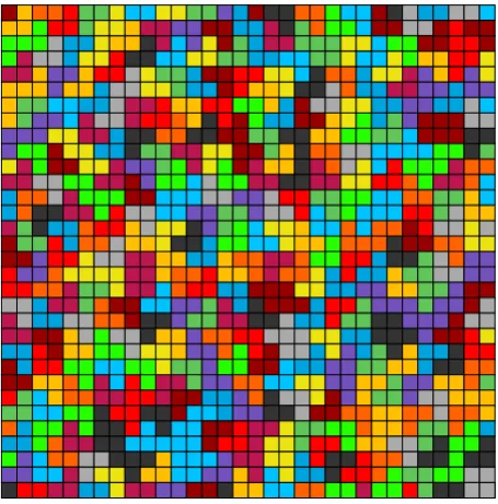
Figure 2.6 shows the structure, numerical results are given in table 2.1.

Figure 2.6: Array structure in the first example

Table 2.1: Output data of the first example

Parameter Value

Number of polyominoes 363

Fullness of the structure A, % 100

Irregularity R 346.36

(59)

Example 2: structure 32 × 32, L-octomino

Input parameters:

• structure size: M = N = 32;

• polyomino type: L-octomino.

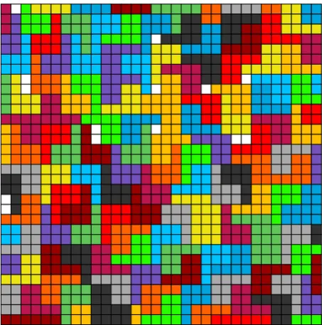
Figure 2.7 shows the structure, numerical results are given in table 2.2.

Figure 2.7: Array structure in the second example

Table 2.2: Output data of the second example

Parameter Value

Number of polyominoes 144

Fullness of the structure A, % 98.63

Irregularity R 370.54

Sidelobe levelγ for r = 1.300, dB −19.97 Sidelobe levelγ for r = 1.818, dB −10.76

Below the analysis of the method is provided from the point of view of

(60)

2.2. DEVELOPMENT OF THE OPTIMIZATION METHOD BASED ON THE STRUCTURE IRREGULARITY ESTIMATION

2.2.2 Colour filtering method analysis

Figure 2.8 shows graphs of irregularity calculated by the colour filtering

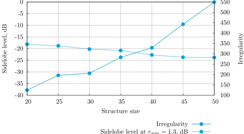
method and sidelobe level obtained by simulation for bandwidthrsim = 1.3.

The experiments were run for structures of different sizes tiled with

L-tromino. Numerical data is presented in table 2.3.

-40 -35 -30 -25 -20 -15 -10 -5 0

20 25 30 35 40 45 50 100 150 200 250 300 350 400 450 500 550 Sidelob e lev el, dB Irregularit y Structure size Irregularity Sidelobe level at rsim = 1.3, dB

Figure 2.8: Irregularity and sidelobe level of st