Large strain computational modeling of high strain rate phenomena in perforating gun devices by Lagrangian/Eulerian FEM simulations

(1)

University of Trento

University of Brescia

University of Bergamo

University of Padova

University of Trieste

University of Udine

University IUAV of Venezia

Luca Gambirasio

LARGE STRAIN COMPUTATIONAL MODELING OF

HIGH STRAIN RATE PHENOMENA IN

PERFORATING GUN DEVICES BY

LAGRANGIAN/EULERIAN FEM SIMULATIONS

Egidio Rizzi (Tutor)

University of Bergamo

2013

(2)

UNIVERSITY OF TRENTO

Doctoral School in Engineering of Civil and Mechanical Structural Systems

Ph.D. Head’s: Davide Bigoni

Final Examination: 29 April 2013

Board of Examiners

Prof. Egidio Rizzi (University of Bergamo, Italy)

(3)

SUMMARY

The present doctoral thesis deals with the study and the analysis of large strain and high strain rate behavior of materials and components. Theoretical, experimental and computational aspects are taken into consideration. Particular reference is made to the modeling of metallic materials, although other kinds of materials are considered as well. The work may be divided into three main parts.

The first part of the work consists in a critical review of the constitutive modeling of materials subjected to large strains and high to very high strain rates. Specific attention is paid to the opportunity of adopting so-called strength models and equations of state. Damage and failure modeling is discussed as well. In this part, specific interest is addressed to reviewing the so-called Johnson-Cook strength model, by critically highlighting its positive and negative aspects. One of the main tackled issue consists in a reasoned assessment of the various procedures adoptable in order to calibrate the parameters of the model. This phase is enriched and clarified by applying different calibration strategies to a real case, i.e. the evaluation of the model parameters for a structural steel. The consequences determined by each calibration approach are then carefullyevaluated and compared. The second part of the work aims at introducing a new strength model, that consists in a generalization of the Johnson-Cook model. The motivations for the introduction of this model are first exposed and discussed. The features of the new strength model are then described. Afterwards, the various procedures adoptable for the determination of the material parameters are presented. The new strength model is then applied to a real case, i.e. a structural steel as above, and the results are compared to those obtained from the original Johnson-Cook model. Comparing to that, the obtained outcomes show that the new model displays a better capacity in reproducing experimental data. Results are discussed and commented.

(4)

(5)

SOMMARIO

Questa tesi di dottorato tratta lo studio e l’analisi del comportamento di materiali e componenti soggetti a grandi deformazioni ed alte velocità di deformazione. Vengono discussi aspetti teorici, sperimentali e computazionali, con particolare riferimento alla modellazione di materiali metallici, sebbene altre tipologie di materiale siano altresì considerate. Il lavoro può essere diviso in tre parti principali.

La prima parte del lavoro consiste in una revisione critica della modellazione costitutiva di materiali soggetti a grandi deformazioni ed alte o molto alte velocità di deformazione. Specifica attenzione è rivolta all’opportunità di utilizzare i cosiddetti modelli di resistenza ed equazioni di stato. La modellazione del danneggiamento e della rottura è altresì discussa. In questa parte, specifico interesse è indirizzato alla revisione del cosiddetto modello di resistenza di Johnson-Cook, sottolineandone entrambi gli aspetti positivi e negativi. Uno dei punti principali presentati consiste in una valutazione ragionata delle varie procedure adottabili ai fini della calibrazione dei parametri del modello. Questa fase è arricchita e chiarificata dall’applicazione delle strategie di calibrazione ad un caso reale, consistente nella valutazione dei parametri del modello per un acciaio strutturale. Le conseguenze determinate da ogni approccio di calibrazione sono poi attentamente valutate.

La seconda parte del lavoro mira ad introdurre un nuovo modello di resistenza, consistente in una generalizzazione del modello di Johnson-Cook. Le motivazioni per l’introduzione di tale modello sono discusse, insieme alle sue principali caratteristiche. In seguito, vengono presentate le varie procedure utilizzabili per la determinazione dei parametri del modello. Il nuovo modello è poi applicato ad un caso reale, l’acciaio strutturale di cui sopra, ed i risultati sono comparati a quelli ottenuti con il modello di Johnson-Cook originale. Comparandosi a tale modello, le previsioni ottenute dimostrano come il nuovo modello presentiuna migliore capacità di riprodurre i dati sperimentali. I risultati sono quindi discussi e commentati.

(6)

(7)

ACKNOWLEDGMENTS

The doctoral candidate thanks his family for supporting the doctoral activities and prof. Egidio Rizzi at the University of Bergamo for tutoring the whole program.

The members of the Board of Examiners are thanked, together with the PhD School Coordinator, prof. Davide Bigoni.

Gratitude is expressed also to prof. David J. Benson at the University of California at San Diego for offering kind hosting and scientific support from September 2011 to July 2012.

Thanks go also to DYNAmore GmbH (Stuttgart, Germany), and in particular to dr. Thomas Münz, for kind hosting and providing a LSTCLS-DYNA license, for a two week period during January and February 2011.

Thanks go to the Lombardia Region, the company TenarisDalmine and the University of Bergamo for granting financial support to this research, through a

(8)

(9)

1

FOREWORD

This doctoral thesis originates from a research program conceived between academia and industry. The research activity has been supported halfway by the Lombardy region, through the University of Bergamo (Department of Engineering, Dalmine), and halfway from the R&D department of the company TenarisDalmine, nearby located. This arrangement has taken place in the context of a regional project called Dote Ricerca Applicata (DRA). Therefore, the targets of the research activity have been established in order to meet the expectations of both academic and industrial partners.

The company TenarisDalmine, strongly involved in the production of seamless pipes and specifically in their applications in the oil and gas industry business, was contacted for possible cooperations on research themes related to computational mechanics. It proposed the analysis and study of a specific device, called perforating gun, which finds use in a critical phase of the extraction process of oil or natural gas from underground deposits, i.e. the radial perforation of rocks and soil surrounding wells. This process allows for and favors the subsequent pumping to the surface of the fluid hydrocarbons. The practical consequences of this perforating phase are of utter importance relatively to the well integrity and productivity. In order to successfully accomplish this process, the perforating gun device plays a role of absolute importance. Hence, the necessity of achieving a good industrial design arises, together with a possible optimization of its key parameters, which may be of different nature, e.g. geometrical, structural, technological or related to the characteristics of the involved materials. The main issue considered in this work regards the structural performance of a particular component of the perforating gun device, technically called carrier.

On the other side, the academic targets were those of achieving original research results in the field of continuum mechanics, with particular reference to large strain and high strain rate behavior of materials. The possibility of proposing some new ideas suitable for the description of such phenomena was evaluated and studied.

(12)

4

Regarding the organization of this work, Chapter 1 briefly introduces some assumptions that are used throughout the exposition. Appropriate considerations about the adopted notation are presented as well. Furthermore, appropriate simplifying assumptions are introduced and motivated.

Chapter 2 presents a brief overview of the constitutive modeling pertinent to large strain and high strain rate material behaviors, in order to critically expose the most popular models suitable for the description of such phenomena. Particular attention is paid to the so-called Johnson-Cook strength model. As a matter of fact, the major part of the presented review deals with this model. This choice is due to the following three main facts. First of all, the Johnson-Cook model appears to be the most implemented and used model when there is the need to model large strain and high strain rate material behavior over a possible wide range of strain rates and temperatures. Second, a new strength model is later introduced in the present work and it actually originates from the Johnson-Cook model, since it considers an enhancement based on the same framework and the same variables. Third, the industrial application examined later in this work makes wide use of the Johnson-Cook model. Different materials are modeled through this specific strength model, although other models are used as well. More in detail, all the key components of the studied perforating gun device are modeled by using the Johnson-Cook model. These salient facts determine the importance of this specific strength model in the context of the present work. The main issue investigated in this section regards a reasoned assessment of the various procedures adoptable for calibrating the parameters of the Johnson-Cook model. This phase is enriched and clarified by applying the calibration strategies to a real case, i.e. the evaluation of the model parameters of a structural steel, by relying on experimental data available from the literature. The consequences determined by each calibration approach are then carefully evaluated, together with a final discussion on the positive and negative aspects of such strategies and some suggestions on how to choose the best calibration approach, by considering the available experimental data and the objectives of the modeling process.

(13)

5

are compared to the results provided by the original Johnson-Cook model. This comparison allows to assess the positive features of the proposed model. The differences between the two compared models are highlighted and discussed. Furthermore, appropriate considerations about the possibility of implementing this new model into FEM codes are pointed-out.

(14)

(15)

7

1. BASIC ASSUMPTIONS AND NOTATIONS

The central aspect analyzed in the present work consists in the large strain and high strain rate constitutive modeling of continuous media, in particular by considering metallic materials. In continuum mechanics, the wording constitutive model tipically refers to a function that relates a measure of strain to a measure of stress, and conversely. Constitutive modeling is one of the most challenging branch of continuum mechanics and its study involves a lot of aspects and considerations. A comprehensive review of these arguments is not an aim of this work. However, it is necessary to point-out some preliminary considerations about a number of basic concepts and notations, as they are adopted throughout the present work.

Ordered arrays of numerical elements are referred to here as tensors, and the number of distinct ordering levels is referred to as the valence or the order of the tensor. A tensor with valence equal to n is denoted by the wording n-tensor. The number of elements in a specific valence is referred to as its cardinality. Given a n-tensor, with n strictly greater than 2, it is said to be a square n-tensor if all its cardinalities are equal.

It is recognized that an abuse of notation may be made here. A n-tensor is indeed something more specific than a simple set of ordered arrays of numbers. Generally speaking, the definition of n-tensor is related to the way in which these numbers describe a quantity in an underlying space and how they transform when passing from one space observer to another. Examples of references on these topics are Levi-Civita, 1926, Struik, 1953, Synge and Schild, 1969, and Moon and Spencer, 1986. Anyway, in order to develop a flowing exposition, the wording n-tensor is used here to refer only to a set of ordered arrays of numbers, without specifying anything particular relatively to its transformation law. This assumption favors simplicity and allows to avoid the involvement of a quite long preliminary treatment of some basic assumptions on which large strain continuum mechanics is implicitly founded, a task that would be too heavy to be presented here and actually not strictly necessary for the achievement of the aims of this work. Furthermore, it appears that this assumption is tacitly assumed in many references, i.e. the wording n-tensor is used in a quite general context, without specifying strict limitations on the transformation rules. Therefore, the approach adopted in the present work allows to fit in this popular framework.

(16)

8

cardinality 3. With further simplification, the space is assumed to be assessed by an observer characterized by having an atlas composed by only one chart. Moreover, this chart is assumed to be Euclidean, i.e. it imposes a metric field gij that is constant in space and equal to the identity 2-tensor, as defined in the following relation

[

]

[

]

[

]

ij ij

1,0,0 g 0,1,0 .

0,0,1

   

= δ =       

(1)

The assumption of imposing an Euclidean metric implies having a vanishing linear connection, denoted by Γ_ijk, as specified in the following equation

lj jk

il lk

ijk ijk

k j l

g g

0 .

2 x x x

_∂ _∂ _∂ 

 

Γ = ⋅_ + − _=

∂ ∂ ∂

 

(2)

As a consequence, any time spatial derivatives are used, the linear connection needs not to be introduced. More specifically, the covariant derivative reduces to the classical derivative. For a treatment on these topics, see, e.g., Marsden and Hughes, 1983, Moon and Spencer, 1986, and Marsden et al., 2007.

Euclidean observers imply the equality of the two natural local bases fields, i.e. the covariant and contravariant local bases field become coincident. This fact leads to the definition of a unique natural local bases field, thus allowing to avoid the need to use subscripts and superscripts in order to distinguish contravariant and covariant n-tensors. Therefore, n-tensors will be denoted by using subscripts only. The choice of limiting the analysis to Euclidean observers only is quite restricting but also favors simplicity and does not hinder the achievement of the targets of the present work.

Functions are denoted by writing first the dependent variable and then the independent variables, gathered by curly brackets and separated by commas. For instance, if A is a function of B and C, the following symbol holds

{ }

A B,C . (3)

(17)

9

Generic evolutions are delimited in time by an initial instant and a current instant. The positions of a point in the initial and in the current instants are denoted by Xi and xi, respectively, and are called initial and current positions, respectively. Motion can then be defined by considering the current position as a function of the initial position and time, as exposed in the following, where time is denoted by the symbol t

{ }

i i

x X ,t . (4)

This function is also called mapping. The deformation gradient, or tangent mapping, is a 2-tensor denoted by Fij and defined in the following way

i ij

j

x

F .

X

∂ =

∂ (5)

The right stretch 2-tensor, denoted by Uij, the left stretch 2-tensor, denoted by Vij, and the rotation 2-tensor, denoted by Rij, arise from the right and left polar decompositions of the deformation gradient, reported respectively in the following equations

3

ij ik kj k=1

F =

∑

R ⋅U , (6)

3

ij ik kj k=1

F =

∑

V ⋅R . (7)

It is also possible to define the velocity of the motion vi, as specified in the following equation

i i

x

v .

t

∂ =

∂ (8)

The velocity gradient is another 2-tensor denoted by Lij and defined as follows

i ij

j

v

L .

x

∂ =

(18)

10

The symmetric part of the velocity gradient is a 2-tensor called rate of deformation and denoted by Dij, while its skew-symmetric part is a 2-tensor called spin and denoted by Wij. Therefore, the following equations hold

(

)

ij ij ji

1

D L L ,

2

= ⋅ + (10)

(

)

ij ij ji

1

W L L .

2

= ⋅ − (11)

It is assumed here that when a 2-tensor is indicated with subscripts arranged inversely to the alphabetical order, the valences indicated by these subscripts are intended as swapped, i.e. the 2-tensor is transposed in these valences. The right stretch and the left stretch allow for defining two sets, each of which is composed by an infinite number of 2-tensors called strain measures. One set defines the so-called Lagrangian strain measures, whilst the other defines the so-so-called Eulerian strain measures. These strain measures are denoted by Eij and Gij and defined respectively by the following relations

m ij ij (m) ij ij U

if m 0

E _m ,

lnU if m 0

 _{− δ}

 _≠ =  ₌  (12) m ij ij (m) ij ij V

if m 0

G _m .

lnV if m 0

 _{− δ}

 _≠

=

 ₌



(13)

The parameter m is assumed to be an integer.

In the present work, a generic strain measure, that could be either Lagrangian or Eulerian, is denoted by the symbol εij. It is possible to decompose any strain measure into its volumetric and deviatoric parts, through the following equation

ij dev vol dev

ij ij ij ij ij

tr , 3

ε

ε = ε + ε ⋅δ = ε + ⋅δ (14)

(19)

11

strain measure εij, it is possible to define an associated scalar quantity called equivalent or effective strain, denoted by ε and defined as follows

3 3

ij ij i=1 j=1 2

. 3

ε = ⋅

∑∑

ε ⋅ε (15)

Sometimes, the equivalent strain is calculated by using a time integral of the rate of deformation, in particular in FEM code implementations. It is then defined by the following equation

3 3

ij ij i=1 j=1 t

2

D D dt . 3

ε =

∫

⋅

∑∑

⋅ (16)

It is worthwhile to point-out that this time integral may not give an equivalent strain attributable to any known strain measure. In this regard, see, e.g. Hoger, 1986.

The time derivative of a strain measure is called strain rate (referred to the considered strain measure) and is denoted by εɺ_ij. Analogously, the time derivative

of an equivalent strain is called equivalent strain rate (referred to the considered

strain measure) and is denoted by εɺ. If elastic and plastic strains are identified, the quantities defined above for a generic strain measure can be specialized to these two cases.

The Cauchy stress is a 2-tensor that stems from considerations on the equilibrium of a continuum body (see, e.g., Bigoni, 2012). It is denoted by Tij and is assumed to be symmetric. It defines a field on a body that describes its stress state. Furthermore, the Kirchhoff stress is another 2-tensor, denoted by τij, still symmetric and defined by the following equation

( )

ij det Fij T .ij

τ = ⋅ (17)

The stress power per unit volume of a continuous body is a scalar denoted by w and defined by the following equation

3 3

ij ij i=1 j=1

(20)

12

It is then said that the Kirchhoff stress and the rate of deformation are work-conjugate variables (see, e.g., Hill, 1978). For each of the previously introduced Lagrangian and Eulerian strain measures, it is possible to define a work-conjugate stress measure. To this end, the next two relations are introduced, in order to define

the so-called Lagrangian and Eulerian stress measures, denoted by T_ij(m) and Z(m)_ij ,

respectively

(m)

3 3 3 3

ij (m) ij ij ij i=1 j=1 i=1 j=1

E

w D T ,

t

∂

= τ ⋅ = ⋅

∂

∑∑

(19)

(m)

3 3 3 3

ij (m) ij ij ij i=1 j=1 i=1 j=1

G

w D Z .

t

∂

= τ ⋅ = ⋅

∂

∑∑

(20)

In the present work, a generic stress measure, that may be either Lagrangian or Eulerian, is denoted by the symbol σij. Analogously to what said for strain measures, it is possible to decompose any stress measure in its volumetric and deviatoric parts, through the following relation

ij ij ij ij ij ij

tr

s p s ,

3

σ

σ = + ⋅δ = + ⋅δ (21)

where the first term in the right member is referred to as deviatoric stress or stress deviator, denoted by sij, and the second term is referred to as volumetric stress. The scalar p is called pressure. Moreover, given a stress measure σij, it is possible to define an associated scalar quantity called equivalent or effective stress, denoted by σ and defined as follows

3 3

ij ij i=1 j=1 3

. 2

σ = ⋅

∑∑

σ ⋅σ (22)

(21)

13

3 3

ij ij 2 i=1 j=1

3

s s s 3 J .

2

= ⋅

∑∑

⋅ = ⋅ (23)

In this equation, J2 represents the second invariant of the stress deviator of the considered stress measure, defined as follows

3 3

2 ij ij

i=1 j=1 1

J s s .

2

= ⋅

∑∑

⋅ (24)

The time derivative of a stress measure is called stress rate (referred to the considered stress measure) and is denoted by σɺ_ij. Analogously, the time derivative

of an equivalent stress is called equivalent stress rate (referred to the considered

stress measure) and is denoted by σɺ .

Furthermore, given a stress measure, it is possible to define a scalar known as stress triaxiality of such stress measure (see, e.g., Meyers, 1994), denoted by x, by introducing the ratio of its pressure and its von Mises stress, as reported in the following equation

p

x .

s

= (25)

The temperature field is denoted by symbol T throughout the work. A final consideration is related to the choice of the strain and stress measures to be related through a constitutive model. In this work, constitutive models are presented in a general way in which strain and stress measures are not forcedly defined a priori. However, when a generic strain measure and a generic stress measure or their time derivative are related through a constitutive model, it is always assumed that they form a couple of work-conjugate strain and stress measures. This hypothesis ensures the fulfillment of some technical requirements which are at the base of the constitutive modeling theory of continuum mechanics.

(22)

(23)

15

2. BRIEF OVERVIEW OF THE CONSTITUTIVE MODELING OF

LARGE STRAIN AND HIGH STRAIN RATE PHENOMENA

Large strain and high strain rate phenomena may be defined as events that occur in a short time, say in the order of fractions of a second, which involve large strains and therefore high strain rates. Plastic strains, damage and fracture are usually present in this kind of processes.

A first aspect of the study of material behavior under dynamic loading involves the analysis of stress wave propagations in solid and fluid materials, for both elastic and plastic regimes. Stress propagates through continuous media as waves with finite velocity. Therefore, a certain time is required in order to allow these waves to spread through the matter. Elastic wave, plastic wave and shock wave propagations are phenomena of utter importance for the study of the dynamic behavior of materials. However, reviewing this entire argument is not on aim of this work. Among others, general treatments are provided in Meyers, 1994, and Wang, 2007. Treatments on elastic wave propagation can be found in Graff, 1965, and Achenbach, 1973. Studies on shock waves and high-pressure shock compression of solids are provided in Asay and Shahinpoor, 1993, Graham, 1993, Horie et al., 2003, Ben-Dor, 2007 and Davison, 2008.

A second key aspect of the study of the dynamic behavior of materials consists in the study of experimental procedures capable to expose the material response to such dynamic conditions. Throughout the years, some particular experimental procedures have emerged over others, thanks to their better feasibility and effectiveness. Dropweight machines, Hopkinson bars, Taylor tests and plate impact tests have become fairly popular. Nowadays, their use is common in many situations, both academic and industrial. Procedures to carry-out these tests and efficiently measure material responses keep on being elaborated and improved as well. A review of these experimental techniques is also not a target of the present work. However, general treatments are provided in Meyers, 1994, and Field et al., 2004. The Taylor test is presented in Taylor, 1948, and Whiffin, 1948. A review on the use of Hopkinson bars is supplied by Jiang and Vecchio, 2009. Some considerations on the procedures necessary to technically execute such tests and relevant test results for different materials are provided in Rajendran and Bless, 1985, and Rajendran, 1992.

(24)

16

contexts involves stress and strain 2-tensor measures as a whole, i.e. it involves the presence of both the deviatoric and volumetric parts. When large strain and high strain rate phenomena are addressed, it is a common practice to decompose these 2-tensors in their volumetric and deviatoric parts and then define two constitutive models, one for the deviatoric part and one for the volumetric part. This practice derives basically from deductions suggested by experimental evidences. An ad-hoc relation between the stress deviator and the strain deviator needs to be established, possibly involving also the strain rate, the temperature and the pressure. Similarly, an ad-hoc relation between the pressure, the volumetric strain and possibly other thermodynamic parameters needs to be established. Basically, the stress deviator is not assumed to be a function of the sole deviatoric strain, in particular when plastic regimes are involved. Similarly, the pressure is no longer a function of the sole volumetric strain. In this context, the wording strength model refers to a function that has the deviatoric part of the stress as dependent variable, while the quite general wording equation of state (also denoted by the acronym EOS) refers to a function that has the pressure as dependent variable.

Beyond strength models and equations of state, an ad-hoc description is also necessary for the modeling of damage and fracture of materials subjected to large strain and high strain rate phenomena. Such models usually need to include the strain rate, the temperature and possibly other parameters. Particular importance is given to the role of stress triaxiality. This parameter does not appear to be widely used in the quasi-static modeling of materials under damage and fracture processes. However, when high strain rates and large strains are involved, the stress triaxiality appears to play an important role in the evaluation of the damage and fracture of the materials.

In the following, some considerations on strength models, equations of state and damage and fracture models are presented, in order to briefly describe the nature of the most used models. In this context, the aim of this chapter is that of analyzing the pertinent literature seeking for the most interesting and successful constitutive models suitable for describing large strain and high strain rate phenomena. Particular reference is made here to the modeling of metallic materials. A brief review of such models and of some references will be made, together with the presentation of some original comments.

2.1. Strength Models

(25)

17

effects of the strain rate and the temperature. Afterwards, many authors have contributed to the development of the knowledge on strength models. In this work, some of the most popular strength models are analyzed and considered, namely the Johnson-Cook model (Johnson and Cook, 1983), the Zerilli-Armstrong model (Zerilli and Armstrong, 1987), the Steinberg-Cochran-Guinan model (Steinberg et al., 1980) and the Steinberg-Lund model (Steinberg and Lund, 1988). These constitutive models are believed to represent some of the most suitable options for the description of high to very high strain rate behavior of materials, in particular for metallic materials, i.e. the materials of highest interest for the industrial application considered in the present research project. More in detail, these models are potentially suitable for the description of materials subjected to the strain rate ranges involved in the considered industrial application. In the following, these models are briefly described and some relevant references are introduced. As previously stated, more attention is paid to the Johnson-Cook strength model, for the following reasons. First of all, it appears to be the most implemented and used material model when there is the need to model large strain and high strain rate material behavior over a possible wide range of strain rates and temperatures. Also, the new strength model introduced later in the present work (Chapter 3) actually originates as an enhancement of the Johnson-Cook model. Furthermore, the industrial application examined later in this work makes wide use of the Johnson-Cook model.

2.1.1. Johnson-Cook Strength Model

The wording Johnson-Cook strength model (also referred to as JC strength model) refers to the hardening function proposed in Johnson and Cook, 1983. The two authors proposed a form for the evaluation of the yield stress as a function of the equivalent plastic strain, the equivalent plastic strain rate and the temperature. Since its first proposal in 1983, this model has gained popularity and nowadays it appears as the most used strength model for the modeling of strain rate dependent phenomena.

(26)

18

Johnson-Cook model to two diverse structural steels. Scapin et al., 2012, presented an application of the model to an alumina dispersion strengthened copper. These are only some illustrative examples of the many applications of the Johnson-Cook model that may be found in the literature.

The Johnson-Cook strength model operates in the classic elastoplastic framework, in which an elastic constitutive model defines the elastic response, a yield criterion defines the delimitation of the elastic regime, and the plastic flow is determined by a flow rule and a hardening function. A review of these classic plasticity concepts is not an aim of this work. Reference is made to, e.g., Hill, 1950, Kachanov, 1971, Lubliner, 2006, and Bigoni, 2012. The Johnson-Cook strength model specifies this classical elastoplastic model by introducing a hardening function capable to model the yield stress dependence on the equivalent plastic strain rate and the temperature. In this context, the Johnson-Cook hardening function is used for updating the stress deviator only. The volumetric response of the material needs to be determined by an equation of state.

When quasi-static regimes are involved, hardening functions are tipically conceived as function of the sole equivalent plastic strain, e.g. through a power function. The contribution presented in Johnson and Cook, 1983, was that of proposing a more general hardening function, suitable for the description of the hardening of materials subjected to large strains, within a certain range of equivalent plastic strain rates and temperatures. Only isotropic hardening was considered, without the introduction of more complicated kinematic or combined hardening rules. Furthermore, one of the main aims of the authors was that of keeping the formulation in a fashion well suitable for implementations in FEM codes.

The form of the proposed hardening function was derived through a totally empiric approach, based on a quite high amount of experimental data collected by the two authors. Tensile and torsion tests were carried-out, considering experimental tests at different strain rates (through an Hopkinson bar) and temperatures. Several metallic materials were tested and analyzed. Results were presented in terms of the Cauchy stress and of the so-called true strain, i.e. the logarithmic strain measure.

On the basis of the obtained experimental results, Johnson and Cook, 1983, introduced a hardening function in which the yield stress manifested a power dependence on the equivalent plastic strain. Furthermore, they pointed-out that the yield stress presented a natural logarithmic dependence on the so-called

(27)

19 p * p 0 p , ε ε = ε ɺ ɺ

ɺ (26)

where εɺ_p represents the current equivalent plastic strain rate and εɺ_p0 represents a

fixed equivalent plastic strain rate, taken as reference value. This value varies accordingly to the available experimental data.

Johnson and Cook, 1983, also pointed-out the fact that the current yield stress exhibited a power dependence on the so-called homologous or homogeneous temperature, denoted by T* and defined as follows

0 m 0 T T T* , T T − =

− (27)

where Tm represents the melting temperature and T0 a fixed temperature, taken as reference value. As for the reference equivalent plastic strain rate, this value varies accordingly to the available experimental data.

On the basis of these observations, the proposed hardening function assumed the following form, in which the yield stress, interpreted as the von Mises stress, is a function of the equivalent plastic strain, the dimensionless equivalent plastic strain rate and the homologous temperature, together with other material parameters

(

n

)

p 0 m

p 0

m 0 p

T T

s A B 1 C ln 1 .

T T

 

 _ε  _ ₋ _

 

= + ⋅ ε ⋅ + ⋅ ⋅ −_ _

 

 _ε  _ ₋ _

   

ɺ

ɺ (28)

The 8 parameters denoted by A, B, n, C, εɺ_p0, T0, Tm and m are referred to as the

parameters of the Johnson-Cook strength model. They need to be calibrated through appropriate experimental tests. Following Table 1 reports their dimensions and possible units.

A Stress, e.g. [MPa] m Non-dimensional

B Stress, e.g. [MPa] εɺ_p0 Strain rate, e.g. [s-1]

N Non-dimensional T0 Temperature, e.g. [K]

C Non-dimensional Tm Temperature, e.g. [K]

Table 1

(28)

20

It is worthwhile to note that the Johnson-Cook hardening function is conceived in a multiplicative fashion, in which the terms contained in the three outer round brackets act together to set the value of the current yield stress.

The first multiplicative term represents a power hardening law, characterized by the three parameters A, B and n. This form is widely used for describing metallic hardening functions in quasi-static modeling contexts. It may then be said that the first multiplicative term represents the quasi-static part of the hardening function and thus it is referred to here as the quasi-static term of the Johnson-Cook strength model.

The second multiplicative term introduces the natural logarithmic dependence on the dimensionless equivalent plastic strain rate and thus it is referred to here as the strain rate term of the Johnson-Cook strength model. This term is conceived in such a way that when the current equivalent plastic strain rate is equal to the reference equivalent logarithmic plastic strain rate it becomes equal to 1 and therefore there are no strain rate effects on the computation of the current yield stress. In such conditions, the hardening response of the material is then ruled by the two other multiplicative terms. Otherwise, the effect of the strain rate on the yield stress is determined by the current value of the equivalent plastic strain rate and ruledby the reference equivalent plastic strain rate and by the parameter C.

The third and last multiplicative term introduces the power dependence on the homologous temperature and thus it is referred to here as the temperature term of the Johnson-Cook strength model. This term is conceived in a way such that when the current temperature is equal to the reference temperature it becomes equal to 1 and therefore there are no temperature effects on the computation of the current yield stress. In such conditions, the hardening response of the material is then ruled by the other 2 multiplicative terms. Otherwise, the effect of the temperature on the yield stress is determined by the current value of the temperature and ruled by the reference temperature, the melting temperature and the parameter m. It is also worthwhile to note that when the current temperature reaches the melting temperature value, this term becomes equal to 0 and thus the current yield stress is assumed to be null and the material is assumed to offer no deviatoric resistance. Temperatures higher than the melting temperature are allowed to occur but then the yield stress is no longer computed with Eq. (28), which would lead to a negative yield stress. In such cases, the yield stress is just set equal to zero.

(29)

21

compromise between simplicity, modeling coherency, requirement of experimental tests and need of computational capacities.

Regarding the positive features of the Johnson-Cook strength model, simplicity and readiness of computational implementation appear to be the most interesting. The model turns-out quite cheap in terms of demand of computational requirements. Furthermore, it is surely well suitable to fit FEM applications, since it uses variables that are readily available in most FEM codes or so-called hydrocodes, namely the equivalent plastic strain, the equivalent plastic strain rate and the temperature. In order to compute the current yield stress, these three variables are the only ones that need to be computed in each timestep of the calculation, since the 8 parameters of the model are fixed and established at the beginning of the calculation. Beyond this aspect, the Johnson-Cook strength model is capable of displaying a good coherence when adopted for the modeling of some basic high strain rate experimental tests, such as for the FEM modeling of Taylor tests. As exposed in Johnson and Cook, 1983, applications of the model in a FEM code (EPIC-2) showed a good matching between the Taylor test computed results and their experimental counterparts. It is often said that the Johnson-Cook model is a formulation able to provide results characterized by having a high enough grade of accuracy, capable to satisfy necessities required in common engineering practices. Actually, these features are the main factors that contributed to the large diffusion of the Johnson-Cook model among the scientific community, in particular towards computational applications.

Regarding the negative aspects, it may be said that the simplicity of the Johnson-Cook strength model is paid by introducing some drawbacks in the formulation. In particular, two main flaws can be identified. The first issue consists in the fact that the natural logarithmic dependence of the yield stress on the dimensionless equivalent plastic strain rate may not be suitable to coherently fit the strain rate dependence of some materials. Analogously, the power dependence of the yield stress on the homologous temperature may present the same shortcoming. These aspects might lead to heavy modeling errors in practical cases.

(30)

22

given temperature, its effect on the yield stress is the same whatever value the equivalent plastic strain and the equivalent plastic strain rate take. The main problem due to this aspect may be the fact that the effects of the equivalent plastic strain rate and the temperature need to be assumed as equal for each equivalent plastic strain. As a matter of fact, this effect may instead be quite different by passing from a condition in which the equivalent plastic strain is null (i.e., the first yielding stress of the material, called also lower yield stress), to conditions with non zero equivalent plastic strain. This point may imply the introduction of heavy coherency errors in the modeling, either of the lower yield stress or of the plastic flow. The more these two aspects present a different dependence on the equivalent plastic strain rate and on the temperature, the more errors are to be introduced, since a compromise between these aspects necessarily needs to be adopted. This simplistic approach may lead to considerable modeling errors, which might actually add to the ones due to the first issue.

At this point, there arise questions about the relevance of these flaws, i.e. how much they may negatively affect the coherency of the model. The point is that of assessing the magnitude of the errors in the prediction of the yield stress for a given equivalent plastic strain, and, accordingly, the magnitude of the errors in the prediction of the equivalent plastic strain for a given yield stress. The examination of the hardening characteristics of the steel adopted in the industrial application under analysis in the present work (i.e., a perforating gun device) suggested that this aspect may be central and heavily affect the computed results, although only a low amount of experimental data was made available. The point here is that the Johnson-Cook hardening function may not be capable to fit the available data with sufficient accuracy in order to produce results fruitfully usable for engineering purposes. Most of all, the fitting may be appropriate only for selected ranges of equivalent plastic strains, equivalent plastic strain rates and temperatures, but not overall.

(31)

23

Johnson-Cook strength model may occasionally introduce heavy modeling errors, in particular when there is the aim of predicting material behaviors over wide ranges of equivalent plastic strain rates and temperatures.

The two previously presented main issues of the Johnson-Cook model did not pass unnoticed in the scientific community. Indeed, the original Johnson-Cook strength model has been the subject of a large number of reviews and modifications. The aims were that of solving or mitigating the negative effects due to the two main drawbacks described above. The following exposition aims at briefly reviewing the main proposed contributions. References that dealt with the first Johnson-Cook issue are presented first, while those which dealt with the second issue are presented second. In this regard, It may be said that the relevance of the Johnson-Cook strength model is further proven by the large number of revisions and enhancements that have been proposed since its first publication.

The first Johnson-Cook issue addresses the fact that a material may not present a natural logarithmic dependence of the yield stress on the dimensionless equivalent plastic strain rate and a power dependence on the homologous temperature. Many authors have contributed to a revision and possibly to a modification of the original Johnson-Cook strain rate and temperature multiplicative terms, in order to improve the coherence of the strength model.

For what it concerns the strain rate term, one of the earlier modifications was presented in Holmquist and Johnson, 1991. These authors pointed-out how the natural logarithmic dependence of the yield stress on the dimensionless equivalent plastic strain rate could be replaced by a power dependence in which the parameter C has now the role of the exponent. In detail, the original Johnson-Cook strength model was substituted by the following one

(

n

)

p C 0 m

p 0

m 0 p

T T

s A B 1 .

T T

 

_ε  _ ₋ _

 

= + ⋅ ε ⋅ ⋅ −_ _

 

_ε  _ ₋ _

   

ɺ

ɺ (29)

This model still uses 8 parameters. Holmquist and Johnson, 1991, presented a FEM implementation of this modified Johnson-Cook model, with the aim of computationally reproduce experimental data from a number of Taylor tests. This modified model provided a better data fitting comparing to the original Johnson-Cook model, although the differences appeared actually marginal.

(32)

24

better account for this effect, the original Johnson-Cook model was modified with the introduction of a power strain rate component added to the natural logarithm strain rate term, leading to a model with 11 parameters, as represented in the following equation

(

n

)

p p k 0 m

p 0 1

m 0

p p

T T

s A B 1 C ln D 1 .

T T

 _ _ _{ } _

ε ε  ₋ 

 _ _ _{ } _

= + ⋅ ε ⋅ + ⋅_ + ⋅ _⋅ −_ _ _ _

  ₋

ε ε

 _ _  _   _

 

ɺ ɺ

ɺ ɺ (30)

In this equation, εɺ_p1 represents an equivalent plastic strain rate value which

determines the transition between the so-called thermally activated regime and the so-called viscous regime. This value was stated to be about 103 s-1. Two further parameters are introduced in the model, denoted by D and k. The modified model was evaluated through numerical simulations of Taylor tests for pure nickel and a high strength nickel alloy. Comparing to the original Johnson-Cook model, the outcomes proved the modified model to display an improved coherency in reproducing experimental data at high equivalent plastic strain rates.

Another modification of the strain rate multiplicative term was proposed by Rule and Jones, 1998. The point was that of modifying the original Johnson-Cook strain rate term, in order to more closely match observed material behavior at high strain rates. Similarly to what stated by Couque et al., 1995, the two authors pointed-out that the yield strength may increase more rapidly with the equivalent plastic strain rates than what determined by the original Johnson-Cook hardening function, in particular for equivalent plastic strain rates that exceed 103 s-1. On this basis, Rule and Jones, 1998, proposed to modify the original Johnson-Cook model in the following way

(

n

)

p 0 m

p 0 1

2 m 0

p p 2 0 p T T 1 1

s A B 1 C ln C 1 .

C T T

C ln

  

   _ _

 _ε   _  ₋  _

= + ⋅ ε ⋅ + ⋅ +  − ⋅ −_ _ _ _

− ε

ε

  ₋  _   _

 _ _

 _ _ε _

  ɺ ɺ ɺ ɺ (31)

(33)

25

of providing a good fit of the yield stress at elevated equivalent plastic strain rates, referring to the capacity of fitting Taylor impact experimental data.

Kang et al., 1999, pointed-out that the original Johnson-Cook strain rate term, which determines a linear dependence of the yield stress on the natural logarithm of the dimensionless equivalent plastic strain rate, may need to be enriched with a term that adds a quadratic dependence of the yield stress on the natural logarithm of the dimensionless equivalent plastic strain rate. This assumption was motivated with reference to some presented experimental data. In particular, it was shown that the quadratic term may be necessary to correctly represent the material behavior at low equivalent plastic strain rates, i.e. rates lower than 1 s-1. The Johnson-Cook hardening function was then modified in the following way

(

n

)

p p 2 0 m

p 0 1 0

m 0

p p

T T

s A B 1 C ln C ln 1 .

T T

 _ _ _{ } _

ε ε  ₋ 

 _ _ _{ } _

= + ⋅ ε ⋅ + ⋅_ + ⋅ _⋅ −_ _

    ₋ ε ε  _ _  _   _   ɺ ɺ

ɺ ɺ (32)

This model uses 9 parameters. A new parameter is introduced in the model, denoted by C1. It determines the weight of the quadratic strain rate term.

Johnson et al., 2006, proposed another modification of the strain rate term by introducing a power term that enriches the modeling of the yield stress dependence on the equivalent plastic strain rate. The following form was then proposed and called high-rate Johnson-Cook model

(

)

C2 m

p p

n 0

p 0 1 0

m 0

p p

T T

s A B 1 C ln C ln 1 .

T T

 _ _ _{ } _

ε ε  ₋ 

 _ _ _{ } _

= + ⋅ ε ⋅ + ⋅_ + ⋅ _⋅ −_ _ _ _

  ₋

ε ε

 _ _  _   _

 

ɺ ɺ

ɺ ɺ (33)

It is worthwhile to point-out that this strength model is a generalization of the model proposed by Kang et al., 1999, i.e. that represented in Eq. (32). This approach introduces two additional parameters, denoted by C1 and C2, leading to a total of 10 parameters. Applications of this model and comparison to the original Johnson-Cook model have been provided in the same reference (Johnson et al., 2006). Referring to the original Johnson-Cook model, the high-rate Johnson-Cook model showed an improved modeling coherency.

(34)

26

(

)

0

m 0

C T T

T T p n m p 0 y p s

s A B 1 1 e .

s

β

 ₋ 

−α_ _

−

 

 

_ε     

   

= + ⋅ ε ⋅ ⋅ + _ − _ 

_ε  _ _ _ _

   

 

ɺ

ɺ (34)

In this equation, s_m, s_y, α and β represent additional model parameters, to be determined from experimental data. The total number of parameters becomes now 11. The two authors presented some applications of the model that demonstrated a more coherent fitting of the experimental data, when comparing to the original Johnson-Cook hardening function, in particular at high temperatures.

Hou and Wang, 2010, introduced a modification of the temperature term in order to better predict the material behavior when the range of temperatures involved is particularly wide. The focus was on a hot-extruded Mg-10Gd-2Y-0.5Zr alloy. Such modified hardening function uses the same 8 parameters of the original Johnson-Cook model. The proposed model is reported in the following equation

(

)

0 m m 0 m T T T T p n

p 0 T

p _T

e e

s A B 1 C ln 1 .

e e

 

 _ε   ₋ 

   

= + ⋅ ε ⋅ + ⋅_ _⋅ − λ

ε  

 _{ } _

−

 

ɺ

ɺ (35)

Other authors presented more complicated developments of the original Johnson-Cook strain rate and temperature terms. As instance, Duc-Toan et al., 2012, introduced a modification of the temperature term in order to enhance the model coherency when very high temperatures are involved.

As proven by the brief review presented here, many modifications of the original Johnson-Cook model have been proposed. In general, it may be said that the first issue of the Johnson-Cook model is partially solved, or mitigated, by the possibility of choosing between different strain rate and temperature terms, with the aim of better fitting the experimental data of the considered material, by taking into account specific equivalent plastic strain rate and temperature ranges. As a matter of fact, some commercial FEM codes allow to choose between some of the different strain rate and temperature terms described above.

(35)

27

marginally. In this regard, some authors proposed modifications capable to partially introduce the synergic dependence of the strain rate and the temperature effects.

For instance, Lin et al., 2010, proposed a modified Johnson-Cook model in which a mixed strain rate and temperature term is introduced. The proposed term is reported in the following equation

(

)

2

(

)

p

1 0 r

p

ln T T p

2

1 p 2 p 0

p

s A B B 1 C ln e .

 _ε 

_{λ +λ ⋅} _{⋅ −}

 _ε 

 

 _ε 

 

= + ⋅ ε + ⋅ ε ⋅ + ⋅ ⋅

 _ε 

 

ɺ

ɺ (36)

The power quasi-static term is replaced by a form that involves a second order trend on the equivalent plastic strain. The parameters B1 and B2 replace the original Johnson-Cook parameters B and n. Their role is that of describing the quasi-static behavior. However, this is only another form to fit data throughout the equivalent plastic strain. The point here is on the strain rate and temperature terms. The strain rate term is maintained the same as in the original Johnson-Cook model. The temperature term is substituted with an exponential term which involves both the dimensionless equivalent plastic strain rate and the temperature. Two new parameters are introduced, denoted by λ1 and λ2, while the parameters Tm and m are no longer present, thus keeping a total number of parameters equal to 8. The proposed model was applied to predict the tensile behavior of a typical high-strength alloy steel, showing a good fitting of experimental data. Furthermore, Wang et al., 2011, proposed a modification similar to the one introduced by Lin et al., 2010, with some variations to the quasi-static and the strain rate terms.

Despite these efforts, the second Johnson-Cook issue appears to be still present, in particular in its heaviest problematics, i.e. the fact that the effects of the equivalent plastic strain rate and the temperature need to be assumed as equal for each equivalent plastic strain, a point which may lead to heavy modeling errors for the prediction either of the lower yield stress or of the plastic flow. In this context, Chapter 3 presents a new formulation capable to mitigate this important shortcoming.

2.2.1.1. Johnson-Cook Model Calibration Strategies

(36)

28

calibration procedure. In this regard, some considerations can be found in Holmquist and Johnson, 1991, but it appears that several key points are still missing. Various other references treated this aspect, such as, e.g., Langrand et al., 1999, Schwer, 2004, Milani et al., 2008, and Scapin et al., 2012, just to cite a few. When it comes to the determination of the 8 Johnson-Cook model parameters, the first aspect to understand is that it is actually possible to define different calibration strategies. In this context, the following exposition aims at reviewing systematically the procedures for the calibration of the Johnson-Cook parameters, a process whose importance is crucial in order to correctly use the model, say at its best potentialities. The most popular calibration approaches are framed, described and discussed, together with the introduction of some original contributions.

(37)

29

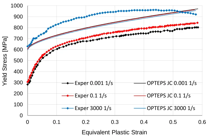
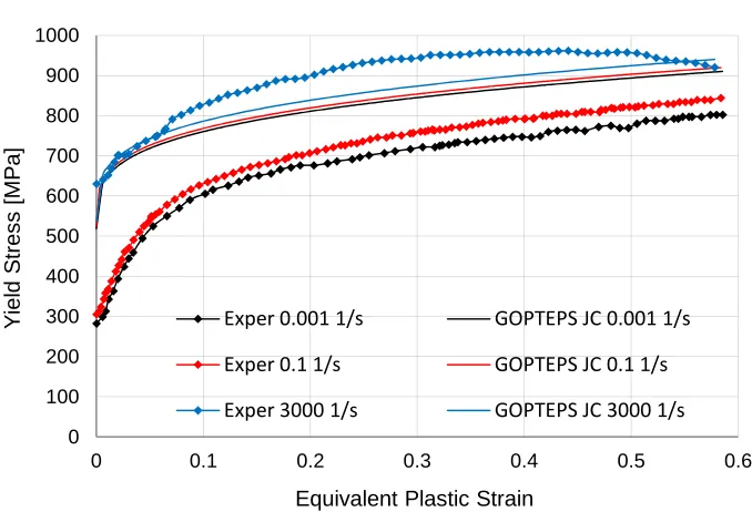
course, this is not an important issue here, since the point under question is only that of showing the outcomes of different Johnson-Cook calibration strategies and not that of fitting the DH-36 steel data as best as possible. Furthermore, data are purified by possible oscillations or peaks near the lower yield stress that may appear in some case, in order to present clearer and more useful data.

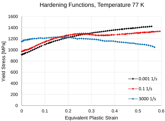
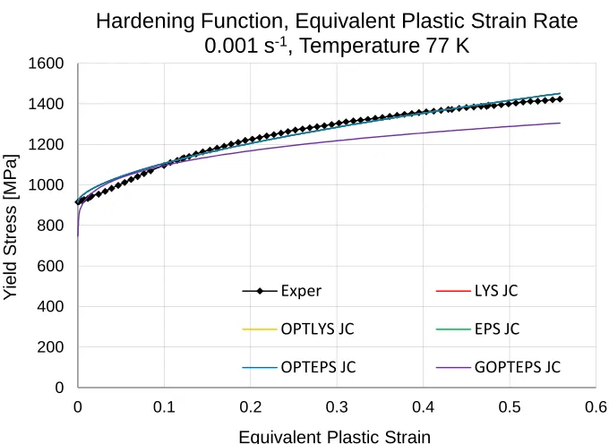
Figure 1. DH-36 structural steel hardening functions at temperature of 77 K and three different equivalent plastic strain rates. Material softening arises for data at 3000 s-1. Data re-elaborated from Nemat-Nasser and Guo, 2003.

0 200 400 600 800 1000 1200 1400 1600

0 0.1 0.2 0.3 0.4 0.5 0.6

Y

ie

ld

S

tr

e

s

[

M

P

a

]

Equivalent Plastic Strain

Hardening Functions, Temperature 77 K

0.001 1/s

0.1 1/s

(38)

30

Figure 2. DH-36 structural steel hardening functions at temperature of 296 K and three different equivalent plastic strain rates. Data re-elaborated from Nemat-Nasser and Guo, 2003.

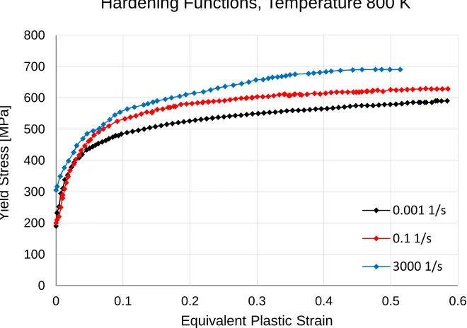
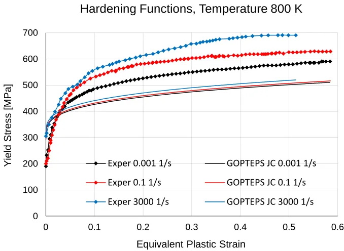
Figure 3. DH-36 structural steel hardening functions at temperature of 800 K and three different equivalent plastic strain rates. Data re-elaborated from Nemat-Nasser and Guo, 2003.

0 100 200 300 400 500 600 700 800 900 1000

0 0.1 0.2 0.3 0.4 0.5 0.6

Y ie ld S tr e s s [ M P a ]

Hardening Functions, Temperature 296 K

0.001 1/s 0.1 1/s 3000 1/s 0 100 200 300 400 500 600 700 800

0 0.1 0.2 0.3 0.4 0.5 0.6

Y ie ld S tr e s s [ M P a ]

Hardening Functions, Temperature 800 K

0.001 1/s

0.1 1/s

(39)

31

Following Table 2 summarizes the lower yield stresses for the nine hardening functions plotted above.

0.001 s-1 0.1 s-1 3000 s-1

77 K 915.555 MPa 974.565 MPa 1150.46 MPa

296 K 282.455 MPa 305.455 MPa 630.137 MPa

800 K 190.345 MPa 200.213 MPa 305.345 MPa

Table 2

DH-36 structural steel lower yield stresses at different equivalent plastic strain rates and temperatures. Data re-elaborated from Nemat-Nasser and Guo, 2003.

It is worthwhile to note that the lower yield stress is strictly increasing with the equivalent plastic strain rate, at each temperature, and that it is strictly decreasing with the temperature, at each equivalent plastic strain rate.

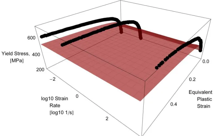
Following Figs. 4 and 5 show the trends of the lower yield stress versus the equivalent plastic strain rate and the temperature, respectively.

Figure 4. DH-36 structural steel lower yield stress versus equivalent plastic strain rate for the three considered temperatures. For representation convenience, the equivalent plastic strain rates are evaluated though their base 10 logarithm. Data re-elaborated from Nemat-Nasser and Guo, 2003.

0 200 400 600 800 1000 1200 1400

-4 -2 0 2 4

L

o

w

e

r

Y

ie

ld

S

tr

e

s

[

M

P

a

]

Log10 Equivalent Plastic Strain Rate

LowerYield Stressvs. Equivalent PlasticStrain Rate

77 K

296 K

(40)

32

Figure 5. DH-36 structural steel lower yield stress versus temperature for the three considered equivalent plastic strain rates. Data re-elaborated from Nemat-Nasser and Guo, 2003.

In the following, five different calibration strategies are described and applied to the just presented experimental data. These approaches appear to be the most intuitive, although it is recognized that they are not the only possible ones and other calibration strategies may be defined. In order to ease their identification, a name is defined here and associated to each of them. The five exposed calibration strategies do not appear to be clearly identified and defined in the pertinent literature. Rather, it seems that different Johnson-Cook calibration strategies are not clearly distinguishable from each other. Thus, the following rigorous and systematic treatment aims at clarifying such situation, at least for the five calibration strategies considered here.

This exposition aims also at introducing some considerations about the experimental tests necessary to get the input for each calibration procedure. In this context, testing the material means to obtain experimental data intended in terms of hardening functions, i.e. curves relating the yield stress to the equivalent plastic strain. Since the Johnson-Cook model does not consider a dependence of the yield stress on the stress triaxiality, these data may come from tensile, compressive or torsion tests, provided that the obtained results are then transformed and evaluated in terms of the von Mises stress and the equivalent plastic strain. However, discrepancies through the parameters may be found when passing from one kind of

0 200 400 600 800 1000 1200 1400

0 200 400 600 800 1000

L

o

w

e

r

Y

ie

ld

S

tr

e

s

[

M

P

a

]

Temperature

Lower Yield Stress vs. Temperature

0.001 1/s

0.1 1/s

(41)

33

test to another, as pointed-out by the original paper that presented the strength model (Johnson and Cook, 1983). This may be related to a dependence of the yield stress on the stress triaxiality, although this appears to be a controversial point and it will not be treated in this work. In this regard, some considerations can be found in Hopperstad et al., 2003, and in Børvik et al., 2003, in which the combined effects of strain rate and stress triaxiality have been investigated.

2.2.1.1.1. LYS Calibration Strategy

The LYS (Lower Yield Stress) calibration strategy aims at determining the set of material parameters capable to achieve the best experimental data fitting for the lower yield stresses, i.e. at null equivalent plastic strain.

The first parameter to be determined is the melting temperature of the material. This phase is straightforward, provided that melting data are available. It is then necessary to identify the equivalent plastic strain rates and temperatures at which it is possible to test the considered material. This information allows to determine the reference values of the equivalent plastic strain rate and of the temperature. Regarding the reference equivalent plastic strain rate, it must be chosen as one of the equivalent plastic strain rates at which the material is tested. No other particular conditions are proposed here, therefore it is possible to choose any of them. A popular choice is that of taking the lowest considered value. Regarding the reference temperature, a sound option is that of taking it equal to the lowest temperature at which the material is tested. This choice is due to the fact that it is necessary to avoid the computation of negative homologous temperatures, since this term is then raised through the parameter m, that may be a non integer number, and therefore the calculation of this power may not be possible. This situation can lead to error terminations when the model is implemented in FEM codes and therefore needs to be avoided. As a consequence, the choice of identifying the reference temperature with the lowest temperature at which the material is tested, in order to avoid this problem. If a FEM simulation is involved, it may also be necessary to check also the fact that the material temperature shall never go below the reference value.

(42)

34

n p

s= + ⋅ εA B . (37)

Under these reference conditions, the parameter A corresponds to the lower yield stress, while the parameters B and n describe the successive hardening of the material. It is then possible to determine the parameters A, B and n by fitting the experimental points with the function shown in Eq. (37). A good strategy here is that of adopting a code that provides nonlinear regression capabilities. Following this strategy, the determination of the three quasi-static parameters, i.e. A, B and n, is due only to the material behavior at the so-called reference conditions, i.e. at reference equivalent plastic strain rate and temperature.

At this point, it is worthwhile to highlight a consideration about the choice of the reference equivalent plastic strain rate. As a matter of fact, the reference equivalent plastic strain rate must be taken as the value at which the quasi-static parameters are evaluated, following the procedure just shown. Otherwise, it is not possible to determine the three quasi-static parameters in the way just exposed, because the strain rate multiplicative term does not vanish. Assuming the reference equivalent plastic strain rate to be equal to 1 and determining the quasi-static parameters by fitting a hardening function which refers to an equivalent plastic strain rate that is actually different from this reference equivalent plastic strain rate may lead to errors. Schwer, 2004, provides a discussion on this aspect, in the context of FEM applicati