Iterative L-M Algorithm in WSN – Utilizing Modifying
Average Hopping Distances
https://doi.org/10.3991/ijoe.v13i10.7006
Xin Qiao, Han-Sheng Yang, Zheng-Chuang Wang Chaohu University, Chaohu, Anhui, China
Abstract—Wireless Sensor Networks (WSN) are getting more and more at-tention for various applications. In addition, localization plays an important role in WSN. This article focus on the large errors of DV-Hop (Distance Vector-Hop) localization algorithm in net topology of randomly distributed notes. A CLDV-Hop (Correct Levenberg Marquardt DV-Hop) algorithm in DV-Hop based on modifying average hopping distances is proposed. Firstly, hop count threshold is to optimize the anchor node during a data exchange. The weighted average hop distance of unknown nodes nearest the three anchor nodes are se-lected as its average hop distance according to the minimum mean square crite-ria. Finally, L-M (Levenberg Marquardt) algorithm is used to optimize the co-ordinate of unknown node estimated by least squares. The simulation results show that, under the conditions of existing overhead and for a given simulation environment, CLDV-Hop algorithm has higher positioning accuracy than exist-ing improved algorithms. The accuracy is improved 33%-41% compared with DV-Hop algorithm.
Keywords—wireless sensor networks, DV-Hop algorithm, localization, L-M algorithm
1
Introduction
Wireless Sensor Network (WSN) consists of a large number of sensor nodes dis-tributed in the area with perceptive, processing and transmitting environment infor-mation. It is often applied in environmental monitoring, medical service, military investigation, industrial diagnosis and intelligent space [1]. Whatever the field is, researches lack of objectives and sensor nodes localization are meaningless. There-fore, node localization technology has become an important research topic in WSN [2].
various positioning algorithms, which can be divided into range-based localization algorithms (Range-Based) and range-free localization algorithm (Range-Free) [4]. The former requires measuring absolute distance and angle between neighboring nodes. The latter can only implement localization, based on the connectivity of the network, such as centroid algorithm [3-5], convex programming algorithm [6], DV-Hop algorithm [7] and Approximate Point-in-triangulation Test (APIT) algorithm [8]. Range-Based has a higher requirement to hardware and it needs repeated measure-ments to obtain reasonable positioning accuracy. Therefore, it will cost a large amount of computation and communication. Range-Free positioning mechanism has been used widely in large-scale WSN with its economization, power-saving and sim-plicity.
DV-Hop is a typical Range-Free localization algorithm with simple implementa-tion and high posiimplementa-tioning accuracy. However, the posiimplementa-tioning accuracy of the pro-posed algorithm is still inadequate in the random distribution of nodes in the WSN. Many scholars have put forward corresponding improvement schemes to solve the problems aiming at high accuracy, stability and efficiency. Reference [9] presented the improved measurement algorithm based on cosamp for image recovery. Reference [10] presented detecting wormhole attacks in Wireless Sensor Networks using hop count analysis. The algorithm set maximum necessary hop count between the sensor nodes and the same neighbor. The algorithm has been improved by above literatures. However, it still cannot meet the requirements of accuracy. Reference [11] proposed using the triangle inequality for constraining the distance from unknown nodes to multi-hop anchor nodes. While using the weighted hyperbolic for positioning. Refer-ence [12] proposed a new method for distance computing from anchor nodes to un-known nodes using the weighted least squares method for location calculation. The CLDV-Hop algorithm proposes and compares with the algorithms in reference [11], [12] through simulation analysis. The results show that the proposed algorithm has higher positioning accuracy and stability in the network topology in randomly-distributed nodes.
2
Algorithm description and error analysis
2.1 DV-Hop algorithm
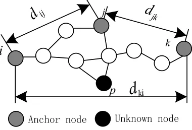
The localization process of DV-Hop algorithm [7, 13] is as follows: The traditional DV-Hop algorithm was put forward by Niculescu and Nath. The basic idea of the algorithm is to estimate distance between the unknown nodes and anchor nodes ac-cording to the product of average per hop distance and hops between unknown nodes and anchor nodes, and then adopt the trilateral law location to obtain the information of node position. Figure 1 illustrates the network topology,
i j k
, ,
represent three anchor nodes,p
represents unknown node.p
k j
i
ij
d
d
jkki
d
Fig. 1. Network structure diagram
First of all, all the nodes in the network receive the hop distance of anchor nodes using the typical distance vector exchange protocol. The nodes can obtain the packet structure as shown in Figure 2. From figure 1, it can be seen that the number of hops among anchor nodes
i j k
, ,
areh
ij=
3
, hjk =4,h
ik=
6
; the hops of unknown nodep
and three anchor nodes areh
ip=
3
,h
jp=
2
andh
kp=
4
.!"#$%&'"%()'
ID
( ,
x y
i i)
hop
''''''''*"+,+-.+/-,+%"'+0'/)&%
Fig. 2. DV-Hop information exchange packet structure
ij j i i
ij j i
d
HS
h
!
!
=
"
"
(1)
Where, ( ) (2 )2
ij i j i j
d = x x! + y y! and ( , ),( , )x yi i x yj j are the coordinates of anchor
i
andj
,h
ij is the minimum hop count between anchori
andj
. For exam-ple, for unknown nodep
in Figure 1, the average hop-sizes calculated byi j
,
and k are 3, 2 and 4 respectively. The average hops distance of anchor nodesi j
,
, andk
are denoted asHS (
i=
d d
ij+
ik) (3 6)
+
,HS (
j=
d
ji+
d
jk) (3 4)
+
and
HS
k=
(
d
ki+
d
kj) / 4 6
(
+
)
.When the average hop distance of anchor nodes is calculated, it is broadcasted to the network through the controlled flooding method. The unknown nodes only record the average hop distance value of the first anchor node. For Figure 1, unknown node
p
receives the average hop distance information from anchor nodej
firstly. There-fore, the distance fromp
to anchor nodesi j k
, ,
are denoted asd
pi=
3 HS
!
j,2 HS
pj j
d = ! and
d
pk=
4 HS
!
j.Finally, when the unknown nodes obtain three or more distance from the anchor nodes, the trilateral positioning method can be executed to solve the estimated coor-dinate of the unknown nodes. Supposing there arenunknown nodes, mrepresents anchor nodes, then the location of unknown node
p
can be estimated through Eq. (2):(2) The above equations can be transformed into
AX b
=
. Among them,A=2 x1!!xm y1!!ym xm!1!xm ym!1!ym
"
# $ $
%
& ' ', b=
x12!xm2+y12!ym2+dm2!d12 !
xm2!!1xm2+ym2!!1ym2+dm2!dm2!1 "
# $ $ $
%
& ' ' '
!X x
y
! " =# $
% & (3)
Therefore, AX b= uses the least squares method to estimate the unknown node
coordinates asX!=(ATA)!1ATb.
2.2 Positioning Error Analysis
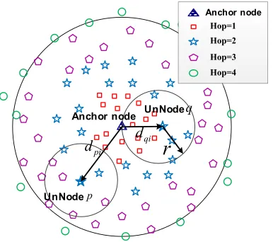
Hop-count information As shown in Figure 3, the network communication model of an anchor node is assumed as a disk shape. Assuming the information nearest the anchor node received by its surrounding unknown nodes as an anchor node in the center of the disk.
d
piis the distance from unknown nodep
to anchor nodei
,d
qiis the distance from unknown nodeq
to anchor nodei
. It can be seen in Fig. 3,h
pi=
h
qi=
2
andd
pi=
HS h
i!
pi , that isd
pi=
d
qi , in factd
qi=
HS h
i!
qi.Therefore, the hop count information brings a lot of errors for the location.Anchor node
r
pi
d
Anchor node
Hop=1 Hop=2 Hop=3 Hop=4
qi
d
p
q
UnNode
UnNode
Fig. 3. Hops and positioning accuracy analysis
The Average Hop Distance: From the process of DV-Hop algorithm in the above, it can be seen that the actual distance between the node and anchor node is the prod-uct of hop count and the average hop distance. Therefore, the positioning accuracy of the whole network is directly affected by the average hop distance. As shown in Fig-ure 3, the WSN nodes are randomly distributed, the route among anchor node
i j k
, ,
is not a straight line, and using average method instead of measuring distance is in-herently existing error. If only using the average hop distance of the anchor node nearest the unknown nodes as the average hop distance to estimate the unknown nodes, the network cannot be reflected wholly.Therefore, the DV-Hop algorithm replaces the distance as the product of the hop count and the average hop distance. The positioning error is not only related to the hop count but also the average hop distance.
calculated through multilateral localization method have greater deviation than real coordinates [14]. In addition, it is found that in the process of simulation, when
A A
T is ill conditioned matrix, the estimated coordinates of unknown nodes not only have large error but the positioning accuracy and stability is also poor through multilateral localization method, sometimes even have incorrect results.3
CLDV-Hop Algorithm
Through the above analysis of the positioning error, the algorithm is improved from three aspects without changing the original algorithm of the structure.
3.1 Weighted average hop distance based on least mean square criterion Traditional DV-Hop algorithm in the calculation of the average hop distance uses unbiased estimation criteria. However, in the randomly-distributed WSN, the error obeys Gaussian distribution. Using mean square error of the average hop distance is more reasonable than deviation or variance [15]. Therefore, this paper uses a least mean square error criterion to calculate the average hop distance, that is:
2
, 1
(
)
N
ij i ij j i i
f
!d HS h
" =
=
%
#
$
(4)
Set 0
i
f HS!
" =
" , the average hop distance of anchor nodes can be presented as:
, 1 2
(
)
N
ij ij j i i i
ij
h d
HS
h
! =
=
"
(5)
In the second stage of DV-Hop algorithm, the average hop distance of the anchor node received by the unknown node is the average hop distance. Considering the distribution of nodes in Wireless Sensor Networks it is not uniformed. Because, only by estimating the average hop distance from a single anchor node to the anchor node around the unknown nodes distance may cause deviation of the local positioning accuracy greatly and the positioning accuracy of the whole network is not stable. Therefore, the positioning accuracy of the whole network can be improved consider-ing the average hop distance of multiple anchor nodes.
If the unknown node can receive the information of
N
anchor nodes, the average hop distance of the anchor nodei
is denoted asHS
i, hops between unknown nodep
and anchor nodei
is denoted ash
pi, and the weight calculation formula based on weighted average hop distance is as follows:1
1
1
pi i Nj pj
h
W
h
=
=
!
(6)
Combined with the network topology of Figure 1, the weight of anchor nodes
, ,
i j k
are4 13
,6 13
and3 13
respectively. Through equation (6), the distance of unknown nodes at different positions in the average hop distance is given different weights. The closer gives larger weight, which can not only reflect the unknown nodes make full use of the recent information of anchor nodes, but also obtain more accurate and reasonable average hop distance. It can be seen from the error analysis of DV-Hop that the accumulated error becomes larger and larger with the increase of hop count. Therefore, choose the average hop distance of the three anchor nodes nearest the unknown nodes as the average hop distance to calculate the average hop distance of unknown nodes. In Figure 1, the average hop distance of the unknown nodes is calculated as,p i i j j k k
C
=
HS W HS W HS W
!
+
!
+
!
(7)According to equation (7), combined with the network topology structure of Figure 1, it can be known that the estimated distance between the unknown node
p
and theanchor nodes can be re expressed as , and .
3.2 Improved threshold based on hop packet format
From the first phase of DV-Hop positioning, it can be known that all anchor nodes send data packets to the surrounding nodes and the format is shown in Figure 2. The anchor nodes send data packets to the surrounding nodes. The nodes of WSN are randomly distributed and the range is uncertain; therefore, the data packets transmit-ted by the anchor nodes are large which leads cumulative error to be larger and larger. To tackle this problem, the data packet format can be improved from the anchor nodes by adding the transmission range of node hops of anchor packet with lifetime limit; that is, the method of limiting the maximum value of the hop count
hop
M. Among them,hop
Mis obtained by multiple simulation experiments. However,hop
M restriction also affects the positioning accuracy directly. Since the smaller the value ofM
In wireless sensor network, anchor nodes information is very important. When there have few or less than three anchor nodes communication, it will lead to lower posi-tioning accuracy and even unable to locate. Therefore, to select appropriate
hop
M, the related factors includes communication radius, the proportion of anchor nodes and wireless sensor network range.!!!!!
!!!!!!!!"#$%$&'$(&%$)#!"*!(+,)
ID
(
x yi, i)
hop
hop
MFig. 4. The modified packet format
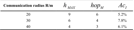
As shown in Table 1, the range of wireless sensor network is the area with 100m*100m and the proportion is 20% with anchor nodes. Communication radius is set as R, the maximum hop count between nodes is
h
MAX, and setting the optimal hop count thresholdhop
M is simulated. The percentage of the positioning accuracy improvement isAc
I compared with the DV-Hop algorithm. The simulation is 100 times, the maximum value is found through the function max (max (Hop1)) each time.h
MAX is the maximum hop count of the 100 times simulation.Table 1. the optimal threshold hops selection
Communication radius R/m
h
MAXhop
MAc
I20 9 6 5.2%
30 6 4 7.8%
40 4 3 6.1%
3.3 Optimal location estimation based on L-M method
Supposing
( , )
x y
is the coordinate of an unknown nodep
, anchor node distance m can be given.( , )
x y
i i is the known coordinate of thei th
' anchor node receiver , andi
d
is the distance from anchor nodei th
' to the unknown nodep
. Supposing there are n unknown nodes, the location of unknown nodep
can be estimated according to equation (8):(x1!x)2+(y
1!y)2=d12
!
(xm!x)2+(ym!y)2=dm2
" # $
% $
These equations can be transformed into
AX b
=
.Therefore,AX b
=
can be solved according to the least square method, and the estimated coordinate of unknown node should be,1
(
T)
! T=
X
A A A b
(9)Convert type (8) into:
2 2 2 2 T
1
( )
m((
i) (
i)
i)
( ) ( )
i
F X
x x
y y
d
X
X
=
=
"
!
+
!
!
=
r
r
(10)In the formula, X is the unknown node coordinate
( , )
x y
, and r( )X is the residual function. Therefore, the estimated coordinates of the unknown nodes can be trans-formed into the unconstrained least squares of equation (10), which is min F(X). L-M method has obvious advantages in dealing with nonlinear least squares optimization. In this paper, the L-M method is used to optimize the method [16]. The iterative for-mula of L-M algorithm can be expressed as:(k1) ( )k
(
( )k)
T(
( )k)
(
(
( )k)
T(
( )k)
)
1(
( )k)
T(
( )k)
X X J X J X µdiag J X J X J X J X
!
+ = !" + #
$ %
& ' (11)
Where,
X
(0) is the initial value( , )
x y
solved by the least squares of the unknownnodes according to formula (7).
k
is the iterative variable,µ
is the damping parame-ter andµ
>
0
. r(X( )k)is,(k) ( ) ( ) ( )
1 2
(X ) ( (
k),( (
k), ,( (
k))
mr X
r X
r X
=
r
!
( )
(X k )
J is the Jacobi matrix consisted of residual function r( )X in the first
deriva-tive at X( )k ,
1 1 1
1 2
2 2 2
1 2 1 2 ( ) ( ) ( ) ( ) ( ) ( ) ( ) ( ) ( ) ( ) m m
n n n
m
r X r X r X
X X X
r X r X r X
X X X
X
r X r X r X
X X X
! ! ! " # $ ! ! ! % $ % ! ! ! $ % $ ! ! ! % =$ % $ % $ % ! ! ! $ % $ ! ! ! % & ' J ! !
" " # " !
(12)
Step1. Obtaining the estimated value Xof unknown coordinate through multilat-eral positioning method and take the estimated value X as the initial value X(0)of
L-M algorithm. Set the damping parameterµ, amplification factor ! and the maximum number of iterations
gx
max, and letk
=
0
.Step2. CalculateF X( ( )k), r(X( )k);
Step3. CalculateJ(X( )k)and calculate!X X= k+1"Xk according to the formula
(11). Determine whether
k gx
>
max is established; if it is established, the optimal solution is X*=X( 1)k+ , iteration ends; otherwise, go to step 4.Step4 If F X( ( 1)k+ ) F X( ( )k)
< , let
µ µ !
=
, go to step 5; otherwise, l=0,letµ µ != " , go to step 5;
Step5 Letk k= +1, go to step 2;
3.4 Process of the CLDV-Hop positioning algorithm
In order to solve the accuracy of DV-Hop algorithm, a wireless sensor network lo-calization algorithm based on the average hop distance correction (L-M) optimization is proposed. The minimum mean square criterion and the weighted hop count are used to estimate the average hop distance to make the result more accurate. Moreover, the hop count is optimized to reduce the accumulated error; meanwhile, the L-M optimi-zation algorithm is used to refine the positioning results iteratively.
CLDV-Hop algorithm steps are as follows:
Step1 Network initialization, at the same time, the simulation related variables are given in this paper (Table 2).
Step 2: Anchor nodes send information by flooding broadcast including its ID, co-ordinates, hops and hop threshold
hop
M.Step 3: Use the shortest path algorithm to compute nodes hop count, calculate the average hop distance of each anchor node through formula (5) and broadcast it to the network and the unknown nodes. Weighted average hop distance is obtained from the nearest three anchors. The distance between unknown nodes and anchor nodes is estimated through the product of the hop count and average hop distance.
Step 4: The least square solution (0)( , )
i i i
X x y of the unknown node
i
is obtained through formula (9).Step 5: Using (0)
( , )
i i i
X
x y
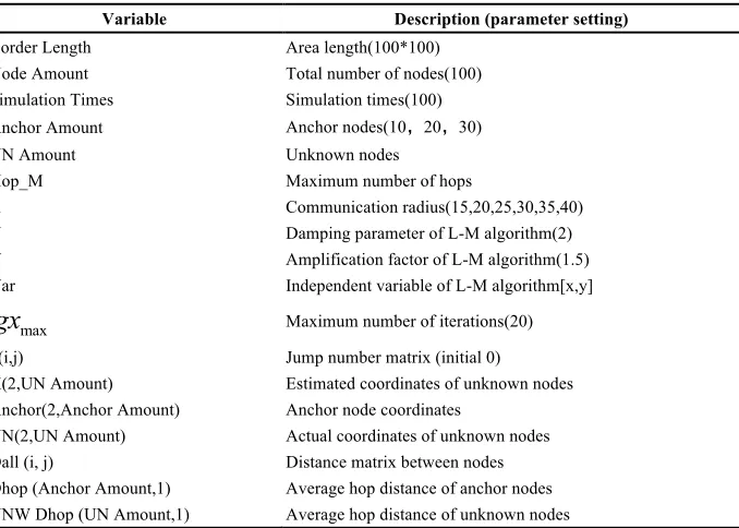
as the initial value of L-M algorithm for iterative re-finement, the estimated coordinate X(2,UN Amount) of unknown nodes is achieved.Table 2. Simulation variables and parameters
Variable Description (parameter setting)
Border Length Area length(100*100) Node Amount Total number of nodes(100) Simulation Times Simulation times(100) Anchor Amount Anchor nodes(102030)
UN Amount Unknown nodes Hop_M Maximum number of hops
R Communication radius(15,20,25,30,35,40) U Damping parameter of L-M algorithm(2) V Amplification factor of L-M algorithm(1.5) Var Independent variable of L-M algorithm[x,y]
max
gx
Maximum number of iterations(20) h(i,j) Jump number matrix (initial 0) X(2,UN Amount) Estimated coordinates of unknown nodes Anchor(2,Anchor Amount) Anchor node coordinatesUN(2,UN Amount) Actual coordinates of unknown nodes Dall (i, j) Distance matrix between nodes Dhop (Anchor Amount,1) Average hop distance of anchor nodes UNW Dhop (UN Amount,1) Average hop distance of unknown nodes
4
Simulation and Experiment
In order to verify the performance of the improved algorithm, it uses 2014b MATLAB platform to simulate and analyze the CLDV-Hop positioning algorithm that proposed in this paper compared with the relevant methods. The other simulation parameters are referenced in table 1.
4.1 Simulation Parameters and Definitions
Network simulation environment settings are that WSN area size is 100x100m, 100 sensor nodes are arranged in the area randomly (including the unknown nodes and anchor nodes). In order to verify the stability of the algorithm, the algorithm sim-ulation has 100 times and take the average value. The relevant definitions involved are as follows,
1.Suppose the actual position of node
i
isT
i, the estimated position isT
!
i. Theaver-age location error of the entire network can be defined ase=
Ti!T!i
i=1
K
"
j=1
N
"
2.Normalized average location errore e r
= : r is the communication radius.
3.To evaluate the performance of algorithms, it usually using the root mean square as a performance measurement of the algorithm. The specific formula is:
2
,
( ( ) ( )) , 1
N
i M M N
e i r i
M N
M N
!
="
= >
" +
#
. (13)
Where,
e i
( )
is an estimated value,r i
( )
is the true value, M is the number of an-chor nodes,N
=
1
.4.2 Algorithm Performance Analysis
Figure 5 is the random distribution of network nodes. Where the red are anchor nodes and the black are unknown nodes.
Figure 6 is thepositioning deviation of unknown nodes which can be seen from Figure 6. Setting the communication radius is 30, the anchor node proportion is 20%, and the improved positioning accuracy is significantly higher than DV-Hop algo-rithm.
Figure 7 and 8 compare with the literature [11], which uses weighted hyperbolic positioning algorithm (denoted as WDV-Hop) and literature [12]. It uses the new algorithm to compute the distance of unknown nodes, anchor nodes (denoted as NDV-Hop) and conventional DV-Hop algorithm. The relationship of the normalized average position error and the total number of nodes of the several algorithms is simu-lated.
In Figure 8, the communication radius is 20,
hop
M is 6, the anchor nodes are 15. It can be seen that, with the increase of the total number of network nodes, the CLDV-Hop algorithm proposed is lower than the average localization error. In Figure 8, the communication radius is 30,hop
M is 4, the anchor nodes are 15. It can be seen that, when the total number of nodes are 150, DV-Hop algorithm error is 9.64, NDV-Hop algorithm error is about 7.24. WDV-Hop algorithm is about 6.95 approxi-mately, while CLDV-Hop algorithm proposed is only 5.96. From Figure 7 and 8, it can be seen that, different communications radius have great impact on positioning accuracy. However, WSN have problems with optimal communication radius and practical application in several tests to select an optimal communication radius.0 10 20 30 40 50 60 70 80 90 100 0
10 20 30 40 50 60 70 80 90 100
Simulation area X axis coordinate/m
Si
m
ul
at
ion ar
ea Y
ax
is
c
oor
di
nat
e/
m
* Red represents anchor nodes ! Black represents unknown nodes
Fig. 5. Random distribution of network nodes
0 10 20 30 40 50 60 70 80
0 5 10 15 20 25 30 35
Unknown node number
Dev
iat
ion di
spl
ac
em
ent
/m
DV-Hop CLDV-Hop
5 10 15 20 25 30 35 10
15 20 25 30 35 40
The ratio of anchor nodes/%
Per
cent
age of
pos
iti
oni
ng ac
cur
ac
y/
%
DV-Hop NDV-Hop WDV-Hop CLDV-Hop
Fig. 7. Localization error varying radio of anchors (R=20m)
5 10 15 20 25 30 35
10 15 20 25 30 35
The ratio of anchor nodes/%
Per
cent
age of
node r
el
at
iv
e l
oc
at
ion er
ror
/%
DV-Hop NDV-Hop WDV-Hop CLDV-Hop
15 20 25 30 35 40 45 50 55 2
4 6 8 10 12 14 16 18 20 22
Relationship between communication radius and positioning error
Communication radius/m
Av
er
age pos
iti
oni
ng er
ror
/m
DV-Hop CLDV-Hop
Fig. 9. Influence of communication radius on positioning accuracy (anchor ratio 20%)
Table 3 is the comparison of the performance between DV-Hop and CLDV-Hop algorithm. The communication radius is set as 30,
hop
M is 4. It can be seen that, the average positioning error of the improved algorithm is much smaller than the tradi-tional algorithm. The positioning accuracy increases about 33%-41% with the differ-ence anchor nodes ratio. The normalized root mean square error of CLDV-Hop is only from 1 3 to1 2
of DV-Hop algorithm. CLDV-Hop algorithm has obvious ad-vantages in positioning performance.Table 3. Algorithm performance comparison
Anchor node Proportion /%
DV-Hop CLDV-Hop
5
Conclusions
This paper proposes iterative algorithm for L-M in WSN, based on modifying av-erage hopping distances. It can be used in large-scale wireless sensor network posi-tioning monitoring with randomly-distributed nodes, such as geological disaster monitoring, water pollution monitoring and forest fire monitoring. The following conclusions can be drawn through the simulation experiment:
1.Problems of the optimal anchor nodes exist in DV-Hop algorithm. Reasonable jump threshold number (rounding far anchor nodes) setting can not only improve the positioning accuracy, but also reduce the amount of communication. The un-known node should communicate with at least three or more anchor nodes.
2.Since DV-Hop localization accuracy can be influenced by average hop distance, the error can be reduced by selecting the weighted average hop distance of nearest three anchor nodes as the average hop distance of the unknown node.
3.Larger errors exist when DV-Hop algorithm uses maximum likelihood estimation or multilateral localization algorithm for over determined equations of least square solution. Higher accuracy can be achieved by transforming into nonlinear least squares optimization and then optimized by L-M.
6
Acknowledgements
The work was supported by Projects of Natural Science Foundational in Higher Education Institutions of Anhui Province (KJ2017A449); Research Fund for the Chaohu University Program (XLY-201603).
7
References
[1]Zhong-min Pei, Yi-bin Li, Shuo Xu. “A fast localization algorithm for large-scale wireless sensor networks”, J Journal of China University of Mining & Technology, Vol. 42(2), 2013, pp. 314-319
[2]En-jie Ding, Xin Qiao, Fei Chang. “Improved Weighted Centroid Localization Algorithm Based on RSSI Differential Correction”, International Journal on Smart Sensing and Intel-ligent Systems, Vol. 7(3), 2014, pp. 1156-1173
[3]Capkun S, Hamdi M, Hubaux J P. “GPS-free positioning in mobile Ad-Hoc networks”, Proc Hawaii International Conference on System Sciences, Maui, HW, USA, 2001, pp. 3481-3490.
[4]Girod L, Bychkovskiy V, Elson J. “Locating tiny sensors in time and space: A case study”, IEEE International Conference Computer Design. 2002, pp. 214–219.
[5]Harter A, Hopper A, Steggles P, “The Anatomy of a Context-Aware Application”, Wire-less Network, 2002, pp. 187-197.
[7]Niculescu D,Nath B, “DV Based Positioning in Ad Hoc Networks”, Journal of Telecom-munication Systems, Vol. 22(1-4), 2003, pp. 267-280.
[8]He T, Huang C D, Blum B M, “Range-Free Localization Schemes for Large Scale Sensor Networks”, Proceedings of the Ninth Annual International Conference on Mobile Compu-ting and Networking San Diego, United states, 2003, pp. 81-95.
[9]G.H.Wu, X.K.Li, J.Y. Dai, “Improved measure algorithm based on cosamp for image re-covery”, International Journal on Smart Sensing and Intelligent Systems, Vol. 7, No. 2, June 2014, pp. 724-739.
[10]Ju Wen, J.X. Jin, Hai Yuan, “Detecting wormhole attacks in wireless sensor networks us-ing hop count analysis”, International Journal on Smart Sensus-ing and Intelligent Systems, Vol. 6, No. 1, February 2013, pp. 209-223.
[11]Ling Zhou, Zhi-wei Kang, Yi-gang He. “Weighted hyperbolic positioning DV-HOP algo-rithm based on triangle inequality”, Journal of Electronic Measurement and Instrument, Vol. 27(5), 2013, pp. 389-395
[12]Min Zhu, Hao-lin Liu, Zhi-hong Zhang, et al. “An Improved Localization Algorithm Based on DV-HOP in WSN”, Journal of Sichuan University (Engineering Science Edi-tion), Vol. 44(1), 2012, pp. 93-98.
[13]En-jie Ding, Xin Qiao, Fei Chang, “Iterative algorithm for Quasi-Newton in WSN based on modifying average hopping distances”, WIT Transactions on Engineering Sciences, Vol. 87, 2014, pp. 589-596.
[14]X Qiao, F Chang, En Jie Ding, “Modifying Average Hopping Distances Based Iterative Algorithm for Quasi-Newton in WSN”, Chinese Journal of Sensors and Actuatiors, Vol. 27, No. 6, June 2014, pp. 797-801.
[15]Wei-wei Ji, Zhong Liu. “Study on the application of DV-Hop localization algorithms to random sensor networks”, Journal of Electronics& Information Technology, Vol. 30(4), 2008, pp. 970-974.
[16]De-min Sun. Engineering optimization methods and applications [M]. Hefei: China Uni-versity of Technology Press, 1997.
8
Authors
Ms. Xin-Qiao, was born in 1988, Suzhou City, Anhui Province, China. She is an Assistant Professor having a Master’s degree. She has been published a number of high-level papers and her research interests are: wireless sensor network positioning technology, ZigBee technology etc. She is with School of Mechanical and Electrical Engineering, Chaohu University, Chaohu, 238000, Anhui, China.
Han-Sheng Yang and Zheng-Chuang Wang are with School of Mechanical and Electrical Engineering, Chaohu University, Chaohu, 238000, Anhui, China.