PhD Dissertation
International Doctorate School in Information and Communication Technologies
DISI - University of Trento
O
N
E
FFICIENT
A
LGORITHMS FOR
S
TOCHASTIC
S
IMULATION
OF
B
IOCHEMICAL
R
EACTION
S
YSTEMS
Vo Hong Thanh
Advisor:
Dr. Roberto Zunino
Universit`a degli Studi di Trento
Abstract
Computational techniques provide invaluable tools for developing a quantitative understanding the complexity of biological systems. The knowledge of the bi-ological system under study is formalized in a precise form by a model. A sim-ulation algorithm will realize the dynamic interactions encoded in the model. The simulation can uncover biological implications and derive further predic-tive experiments. Several successful approaches with different levels of detail have been introduced to deal with various biological pathways including regu-latory networks, metabolic pathways and signaling pathways. The Stochastic simulation algorithm (SSA), in particular, is an exact method to realize the time evolution of a well-mixed biochemical reaction network. It takes the inherent randomness in biological reactions and the discrete nature of involved molec-ular species as the main source in sampling a reaction event. SSA is useful for reaction networks with low populations of molecular species, especially key species. The macroscopic response can be significantly affected when these species involved in the reactions both quantitatively and qualitatively. Even though the underlying assumptions of SSA are obviously simplified for real bi-ological networks, it has been proved having the capability of reproducing the stochastic effects in biological behaviour.
reactions have to update their propensities to reflect the changes.
In this thesis we investigate new algorithms for improving performance of SSA. First, we study the application of tree-based search for improving the search of a reaction firing, and devise a solution to optimize the average search length. We prove that by a tree-based search the performance of SSA can be sen-sibly improved, moving the search from linear time complexity to logarithmic complexity. We combine this idea with others from the literature, and compare the performance of our algorithm with previous ones. Our experiments show that our algorithm is faster, especially on large models.
Second, we focus on reducing the cost of propensity updates. Although the computational cost for evaluating one reaction propensity is small, the cumula-tive cost for a large number of reactions contributes a significant portion to the simulation performance. Typical experiments show that the propensity updates contribute 65%to85%, and in some special cases up to99%, of the total simu-lation time even though a dependency graph was applied. Moreover, sometimes one models the kinetics using a complex propensity formula, further increasing the cost of propensity updates. We study and propose a new exact simulation algorithm, called RSSA named after Rejection-based SSA, to reduce the cost of propensity updates. The principle of RSSA is using an over-approximation of propensities to select a reaction firing. The exact propensity value is evaluated only as needed. Thus, the propensity updates are postponed and collapsed as much as possible. We show through experiments that the propensity updates by our algorithm is significantly reduced, and hence substantially improving the simulation time.
Third, we extend our study for reaction-diffusion processes. The simulation should explicitly account the diffusion of species in space. The compartment-based reaction-diffusion simulation is compartment-based on dividing the space into
subvol-umes so that the subvolsubvol-umes are well-mixed. The diffusion of a species between
new algorithm, called Rejection-based Reaction Diffusion (RRD), to efficiently simulate such reaction-diffusion systems. RRD combines the tree-based search and the idea of RSSA to select the next reaction firing in a subvolume. The high-light of RRD comparing with previous algorithms is the selection of both the subvolume and the reaction uses only the over-approximation of propensities. We prove the correctness and experimentally show performance improvement of RRD over other compartment-based approaches in literature.
Finally, we focus on performing a statistical analysis of the targeted event by stochastic simulation. A direct application of SSA is generating trajectories and then counting the number of the successful ones. Rare events, which occur only with a very small probability, however, make this approach infeasible since a prohibitively large number of trajectories would need to be generated before the estimation becomes reasonably accurate. We propose a new method, called
splitting SSA (sSSA), to improve the accuracy and efficiency of stochastic
sim-ulation while applying to this problem. Essentially, sSSA is a kind of biased simulation in which it encourages the evolution of the system making the target event more likely, yet in such a way that allows one to recover an unbiased es-timated probability. We compare both performance and accuracy for sSSA and SSA by experimenting in some concrete scenarios. Experimental results prevail that sSSA is more efficient than the naive SSA approach.
Keywords
Acknowledgments
I would like to thank my supervisor Roberto Zunino. I am indebted to him very much for his countless help and support. He always has time for me to listen and give me useful advice in my journey in science.
Contents
1 Introduction 1
1.1 Biological modelling and simulation . . . 1
1.2 The need and challenges for stochastic simulation . . . 3
1.3 The objective of the thesis . . . 7
1.4 Structure of the thesis . . . 10
2 Stochastic Simulation: A Literature Review 11 2.1 Introduction . . . 11
2.2 Reaction network representation . . . 16
2.2.1 Coupled reaction list . . . 16
2.2.2 Graphical network diagram . . . 17
2.3 Simulation algorithm . . . 19
2.3.1 Exact stochastic simulation . . . 19
2.3.2 Approximate stochastic simulation . . . 29
2.3.3 Hybrid stochastic simulation . . . 33
2.3.4 Stiff system simulation . . . 36
2.3.5 SSA Extensions . . . 39
3 Tree-based search 43 3.1 Introduction . . . 43
3.2 Complete Tree Search . . . 44
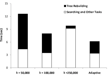
3.3.1 Fixed time tree rebuilding . . . 50
3.3.2 Adaptive time tree rebuilding . . . 55
3.4 Conclusion . . . 58
4 Rejection-based update 61 4.1 Introduction . . . 61
4.2 RSSA . . . 63
4.2.1 Selection of reaction firing . . . 64
4.2.2 Reaction firing time . . . 68
4.2.3 The RSSA algorithm . . . 70
4.2.4 Proof of correctness . . . 73
4.2.5 Fluctuation interval control . . . 76
4.3 Experimental results . . . 79
4.3.1 Fully connected reaction model . . . 81
4.3.2 Multiscaled reaction model . . . 84
4.3.3 Gene expression model . . . 85
4.4 Towards an Optimal Parameter Selection . . . 90
4.5 Conclusions . . . 94
5 Rejection-based reaction diffusion 97 5.1 Introduction . . . 97
5.2 Reaction-diffusion simulation . . . 100
5.2.1 Spatial SSA . . . 100
5.2.2 Rejection-based reaction-diffusion simulation . . . 102
5.2.3 The RRD algorithm . . . 104
5.2.4 Correctness of the RRD algorithm . . . 107
5.3 Experimental results . . . 108
5.3.1 cAMP activation of PKA model . . . 110
5.3.2 Multiscaled reaction-diffusion model . . . 112
6 Rare event probability estimation 117
6.1 Introduction . . . 117
6.2 Problem setting . . . 119
6.3 Splitting for rare event simulation of reaction networks . . . 121
6.3.1 Splitting approach . . . 121
6.3.2 Choosing a level function . . . 125
6.3.3 The sSSA algorithm . . . 126
6.4 Experimental results . . . 129
6.4.1 Production degradation model . . . 130
6.4.2 Biological switch model . . . 136
6.5 Conclusions . . . 138
7 Conclusion 141
Chapter 1
Introduction
1.1
Biological modelling and simulation
Recent advances in molecular biology have been doubtlessly continuing and increasing our knowledge of biological systems. The detailed quantitative data produced allow to characterize, for example, the entire human genome sequence and its products [144]. However, genes, proteins and their interconnections alone are not sufficient to explain all the complexities of living organisms. A cellular system, in essence, is a dynamic system in which its functions are not controlled only by the network structure but also the dynamics of involving elements. Explaining how the molecular interactions and, at its best, the combi-nation principles emerging to a specific cellular behaviour needs a system-wide perspective. The cell differentiation during the cell cycle is just an example. By changing the experiment conditions, e.g., initial conditions, stimulus, the resulted cells can be very different, even counter-intuitive patterns. This is due to the dynamic characteristics and non-linearity of this process. A system level analysis of biological systems is thus a promising approach to provide an insight explaining of biological phenomena.
Systems biology is an emergent research area as a combination of system
rise to a specific behaviour at the system level, and ultimately, to develop new biological systems for useful purposes e.g., effective prevention and/or treat-ment of diseases (see e.g. [87–89, 173] and references therein).
The computational modelling and simulation plays an important role in the development of systems biology in twofold. First, it abstracts out a biological network in term of a model. The model encodes the temporal evolution of its
state in a formal form. Second, it allows to visualize and to predict the
causal-effect of the biological system in time through a computer simulation.
Essentially, a model is an effort to explicitly encode the knowledge of bio-logical system in a precise form. Depending on features of the biobio-logical sys-tem under study, the model should include sufficient information for analyzing the system dynamics. For example, at a detail molecular modelling, the model should manage all the detailed information, e.g., velocity and/or position, of all molecular species. A whole-cell model, in contrast, should include only a de-scription of all key cellular processes. A biological model, to some extent, is therefore just an abstraction of the real system; however, it is useful to formalize the understanding of the biological system. So, modelling provides an effective way to highlight gaps in knowledge of biological systems.
extremely useful for doing quantitative analysis of biochemical systems.
The biological modelling and simulation further contribute to the design and implement. A component-based approach is more effective than build-ing the entire system from scratch, which is often more error-prone. The well-understood models with detailed interacting behaviour are reused as basic build-ing blocks in a large model. The substitutable feature of this approach provides an opportunity to reprogram cellular functions to serve for special purposes of biological research [160].
Summing up, biological modelling and simulation in the post-genomic era are becoming increasingly important. The knowledge of biological system is able to integrate into a model, and make testable predictions through simulation. In silico experiments, in this sense, are highly preferred in term of speed, ease and cost; however, it is also important to emphasize that in silico experiments cannot be considered as a substitution of real biological experiments. In silico experiments thus are used in complement to biological research.
1.2
The need and challenges for stochastic simulation
Different levels of modelling and simulation detail have been adopted to in-vestigate the dynamics of biological systems. At higher coarse-grained level the deterministic approach, where the concentration of molecular species are considered, has the capability of predicting dynamic behaviour of biochemical systems. The application of deterministic approach often lies on the law of mass
action which states the rate of a reaction is directly proportional to the
Furthermore, a lot of well-developed tools, e.g., stability and bifurcation anal-ysis [150], metabolic control analanal-ysis (MCA) [53], have been introduced for analyzing the behaviour of ODE.
The law of mass action has been successful to model chemical reactions at equilibrium (see [42, 73] for examples); however, its underlying assumption is obviously oversimplified for biological systems. The changes in population of molecular species due to reaction firings are assumed to be less significant so that population of molecular species are considered as continuous. The fluctu-ations of involved species, in this sense, have a negligible effect to the macro-scopic trend of the molecular concentrations. Thus, the law of mass action describes only average behaviour. The molecules involved in biochemical reac-tions, however, are obviously discrete. Furthermore, it is common to find in a model few specific species, e.g., genes, mRNAs, which play a key role, yet have a very small population. Small changes in these species can lead to a significant quantitative and qualitative fluctuation in the behaviour of the overall biological system. Second, a collision between molecular species to form a reaction is inherently random. The occurrence of a random reaction can give rise to un-expected responses, e.g., bistability response pattern. Such random fluctuations at molecular level are inevitable and referred to as biological noise. The im-portant of the fluctuations and noise in biological systems have been repeatedly pronounced in recent research (see e.g., [9,46,108,109,127,158,166]). The ran-dom effects in such systems can help to explain many biological phenomena, e.g., phenotypic variants [131]. Finally, biological noise itself has an important role in enhancing inter- and intra-cellular functions. The noise is propagated from cell to cell to modulate and improve the cellular signaling [122, 130]. A quantitative understanding of biological responses taking account of stochastic effects is preferred.
the most detailed and accurate method. It has to keep tracking all the positions, velocities as well as possible collisions of every molecules in the biological sys-tem. Although this approach yields an accurate result, it requires a very detailed knowledge of the molecules both in time and space, and computationally inten-sive in performing simulation. Hence, MD is limited to simulate the system only at the nanoscale of time and/or space. The stochastic kinetics is a more practical approach that still could capture the stochastic noise. In stochastic ki-netics, the system state is denoted by a vector of population of species. Species can interact through coupled biochemical reactions. A reaction firing will cause the system state to move to a new state.
The stochastic kinetics is underpinned on that the probability a reaction firing in the next infinitesimal time can be expressed by a propensity function. In [60] a derivation for the existence of such propensity function for the so-called
ele-mentary reaction, which involves at most two molecular species as reactants, is
provided. The dynamic time evolution of the reaction network thus can be de-scribed as a (continuous) jump Markov process. A complete mathematical form for expressing the time evolution of the system state is generally referred to as
Chemical Master Equation (CME) [64]. A directly analytic solution of CME,
however, is hard to obtain unless the system is very small. Fortunately, we can construct an exact realization of CME through a simulation method called
stochastic simulation algorithm (SSA) [60, 61, 65]. SSA realizes a possible state
transition by randomly selecting a reaction to fire according to its propensity. At the new state, affected reactions have to update their propensities to reflect the changes.
design and control. The simulation time of a SSA run is mainly dominated by two sources: search for the next reaction firing and update the propensities after a reaction fired. First, an inefficient search for the next reaction firing such as the linear search is asymptotically increasing with the number of re-actions in the model. The linear characteristic thus limits the application of SSA to large models. Second, a large model is typically encompassed with a large number of interconnections and (feedback) loops. The propensity up-dates required anytime the population of involved species is changed are also a computational bottleneck. Moreover, sometimes one models the kinetics using a complex propensity formula, e.g., the Michaelis-Menten equation, the Hill equation, further increasing the cost of propensity updates. The computation cost of SSA is further increased when relaxing the underlying assumptions of SSA. For example, to handle the movement of species in space, the extension of SSA is introduced by dividing space into subvolumes. A species can locally interact with other species inside a subvolume or jump to its neighbors. The search and update of reactions obviously take more computational demand be-cause the number of species and reactions grow with the number of subvolumes. Due to the stochastic behaviour in a single realization, a lot of simulation tra-jectories are required to ensure correct statistical information of the final reach-able states. For example, to estimate the reaching probability of a given set of targeted states, one needs to generate an ensemble of independent SSA simu-lations (say 106 runs) and count which hits the target to collect a reasonable
statistics. SSA will soon become inefficient to estimate the rare event proba-bility since a prohibitively large number of trajectories, and of course very high computational effort, would need to be generated before the estimation becomes reasonably accurate.
In particular, in stiff system, the fast reactions occurs frequently and drive the system into stable state very fast. After this short fluctuation time, the slow reactions will determine the system dynamics. However, most of the time the simulation samples the fast reactions which is not the expected behaviour of the system. Furthermore, the population of some species involved in reactions may also many orders of magnitude larger than others. The fluctuations of these species, when reactions fire, are less significant. Keep tracking single reaction firings for large population species by SSA is obviously less efficient since a coarse-grained simulation method can be applied without loss of total simula-tion accuracy. Because of the inherent dynamics in biochemical reacsimula-tions, a model can combine and mix all of these aspects in a very complicated man-ner. For example, the system exhibit stiffness at beginning, but then requires to consider a single reaction firings. It also can start with large population of some species then their population become small because of many reactions fir-ings. These issues raise a great challenge for developing and implementing of an efficient stochastic simulation method [142, 154].
1.3
The objective of the thesis
In this thesis we aim to improve the existing methods and investigate new algo-rithms for efficiently performing exact stochastic simulation. We contribute to the improvement of SSA in following aspects:
study efficient approaches to rebuild the tree when it becomes non-optimal. • We study the effect of the propensity updates to the overall performance of stochastic simulation. Even though a dependency graph can reduce the propensity updates to be model-dependent, in which only locally af-fected reactions have to recompute their propensities, still there are mod-els, e.g., highly coupled reactions, where costly updates are required. The update cost is further increased if a complex propensity function is ex-ploited to model complex effects, e.g., the allosteric effect in modelling protein binding mechanism. The simulation time is significantly affected by propensity updates. We propose a new algorithm, called RSSA, to avoid fully recomputing propensities of affected reactions as much as possible. RSSA uses an over-approximation of propensities to select a candidate re-action. The candidate reaction is then subjected to a rejection-based proce-dure to decide either accept this selected reaction to fire or (with low prob-ability) reject it. We experimentally study different search procedures for finding a candidate reaction and discuss which leads to better performance, for different network sizes. We subsequently study several strategies for controlling the amount of over-approximation (hence, indirectly the accep-tance probability), and analyze their impact to the simulation performance. We also discuss how to systematically optimize the tunable parameters of RSSA so to maximize its performance.
reactions. As a result, the number of species and reactions in a reaction-diffusion model are increased linearly with the number of subvolumes. The simulation thus requires a prohibitive computational cost for both of the search of a reaction firing in a subvolume and the update of affected reactions and subvolumes after a reaction fired. We contribute to this topic by proposing a new method called RRD. RRD combines the tree-based search and the principle of RSSA to improve performance of the stochas-tic reaction-diffusion simulation. First, a candidate subvolume is selected through a binary search on an over-approximation of subvolume propen-sities. Then, a candidate reaction in this subvolume is retrieved by using a fast lookup search on an over-approximation of reaction propensities. A rejection-based procedure is finally applied to either accept the reaction to fire or reject it. These features of RRD make it scale well with both large numbers of subvolumes and reactions.
1.4
Structure of the thesis
The outline of the thesis is the following.
In chapter 2 we briefly review modelling techniques to represent a biochem-ical reaction network. Then, we give a detailed review of stochastic simulation techniques, including exact, approximate and hybrid methods to improve the performance of SSA. The extensions of SSA obtained by relaxing its underlying assumptions i.e., reactions with delayed time and spatiality, are also reviewed.
In chapter 3 we describe in detail the application of tree-based search to improve the search of next reaction firing. The underlying data structure and algorithm for performing binary search are detailed. Then, we study which tree structures leading to an optimal search length and tree rebuilding strategies when the tree becomes non-optimal. A part of this chapter has been published in [156], of which an extended version is submitted for publication.
In chapter 4 we present key steps of RSSA for finding a reaction firing with its firing time based on the over-approximation propensities. We provide a for-mal proof for the correctness of RSSA. Then, we discuss different search pro-cedures for finding a candidate reaction supported by RSSA as well as several mechanisms to control the amount of approximation, hence controlling the ac-ceptance probability. A part of this chapter has been submitted for publication.
In chapter 5 we will describe in detail the RRD algorithm. The key steps for selecting a subvolume and a reaction firing in that subvolume are presented. A proof for correctness of RRD is also presented.
In chapter 6 we formulate the problem of rare event probability estimation in the stochastic simulation setting. Then, we present the sSSA algorithm and its features for improving the efficiency and accuracy of estimating the probability of rare events. A part of this chapter has been published in [157].
Chapter 2
Stochastic Simulation: A Literature
Review
2.1
Introduction
Molecular species, e.g., genes, mRNAs, proteins, are constantly moving inside a cell. Following a species trajectory, it can collide with other species. A colli-sion between molecular species will form a reaction if it satisfies some specific conditions, e.g., activation energy, which are known as the reaction kinetics. The rate of a reaction, in essence, depends on a rate constant and reactants. The result of a reaction is new molecular species produced to help performing necessary activities of the cell. The reaction pathway is an organized reaction network to perform special cellular purposes. A biological system exploits dif-ferent pathways by many mechanisms, e.g., feedback and feedforward loops at different levels, e.g., time and/or space to control, regulate and coordinate op-erations between cells. The understanding of these mechanisms becomes more difficult when random noise, yet important, is taken part in these processes. The stochastic framework provides promising tools for performing an insight analysis of the system behaviour at system-wide level.
of the reaction network as well as its parameters in a more formal, precise and testable form. It must be simple, flexible and scalable enough for modelling different types of reaction networks ranging from very small, e.g., simple gene expression, to very large, e.g., complex signaling pathways, metabolism or even living organisms. Further, the model should be standardized so that it is able to share information, data and knowledge between communities. Second, a sim-ulation algorithm is built to visualize the time evolution of the system. The simulation should be able to capture important features in the dynamics of bi-ological processes. It also takes into account bibi-ological noise as an important factor affecting the system evolution. Thus, the grand challenge in computa-tional biology is to model and simulate a full cellular organism [142, 154].
concurrently through channels. A logical process could be implemented as an instance of a runnable process in a computer, so it is easy to turn an entire model into an executable simulation. Furthermore, these formalisms have strong and well-studied mathematical background. A lot of well-developed mathematical tools have been developed to support for useful analysis, e.g., checking equiv-alence behaviour, model checking [1, 113]. New modelling techniques such as rule-based modelling [50, 107, 146], also get more attention recently. They are introduced to overcome the explosion problem in modelling reaction path-ways, e.g., signaling pathway. For example, in rule-based modelling, reactions are modelled as rules. A rule also encompasses with extra information for the reaction firing, i.e., reaction kinetics. If a rule is matched, the corresponding reactions is introduced to the system at runtime. Thus, all the possible reactions in the model do not need to be specified at the beginning of simulation.
for performing biochemical simulation. These algorithms can count for the stochasticity in time and/or space.
For a well-mixed biochemical reaction system, the stochastic simulation al-gorithm (SSA) [60, 61] is a de facto standard for numerically sampling the time evolution of a biochemical reaction network. The development of SSA has the mathematical background on the chemical master equation (CME) [64], which completely describes the probability distribution of all possible state transitions. SSA takes into account the inherently random fluctuation of the involved molec-ular species as a main source in selecting a reaction firing. It is an exact method in the sense it does not introduce any source of approximation in selecting the reaction. In other words, it gives the same result as the analytic solution of CME, while the later is intractable for many cases. Essentially, SSA searches for a reaction to fire at a time based on a probability function. The reaction probability distribution depends on the (current) system state and the chemical kinetics. Anytime a reaction fires, the system configuration, i.e., the system state, as well as the reaction probability distribution have to be updated.
approxi-mate method is theτ-leaping [63] algorithm. Although approximate algorithms indeed run faster, they expose serious problems especially to models having just some species at very low copy numbers. Firing many reactions in one time step yields the negative population for these species which is obviously infeasible in real experiments. A promising approach to solve this problem is the hybrid sim-ulation [121]. It treats the system by two complementary parts. The part with low population species is simulated by an exact stochastic simulation, while the part with the high population species is treated by a fast simulation algorithm e.g., ODE integration, τ-leaping. Hence, it still achieves a better performance and also captures the important stochastic effects.
The assumptions of SSA, e.g. instantaneous reaction firing, well-mixed so-lution, is restricted for living cells. The effects of these factors when consider-ing can alter the behaviour of the biological network significantly. Hence, SSA should be adapted to account for these factors. For example, the highly localiza-tion of species which is generally referred to as the molecular crowding [33, 82] enhances the availability of species, and thus speeding up the operations of cellular processes. It also helps to explain important effects in biological sys-tems, e.g., the excluded volume effect. Thus, taking spatial information into the stochastic simulation is a crucial task [153]. A possible extension of SSA for spatially heterogeneous environment is dividing space into well-mixed subvol-umes. The diffusion of a molecular species between subvolumes is explicitly modelled by an additional unimolecular reaction. The extension of SSA in this manner is known as the compartment-based simulation.
simula-tion algorithm. Then, we are going to details of the algorithms for conducting stochastic simulation of biochemical reaction networks. We cover fundamental ideas of SSA as well as efficient formulations proposed during the time course. We also present a brief review of approximate and hybrid methods to improve the performance by the cost of its exactness. The extensions of SSA by relax-ing the underlyrelax-ing assumptions of the biochemical reaction networks are also reviewed. Two possible extensions are reviewed namely: reactions with delays and reactions with spatiality.
2.2
Reaction network representation
2.2.1 Coupled reaction list
Listing all the reactions in the network is a direct way to specify reactions of the model. The network thus will be expressed in form of coupled reactions. Let consider a biochemical reaction system consisting n species denoted as
S1, ...Sn. These species interact through m reactions R1, ...Rm. Each reaction
has the following general form:
Rj : v1jS1 + ...+vnjSn kj
→v1′jS1 +...+vnj′ Sn (2.1)
where vij and vij′ are referred to as stoichiometric coefficients. In fact vij is
the number of species Si are consumed and, in contrast, vij′ is the number of
species are produced by reaction Rj. In this general reaction form, we allow
some species to appear in the both side of a reaction. The appearance of such species is only to increase the rate of the reaction and this species is generally called a catalyst. kj is the (stochastic) rate constant of reactionRj. A reversible
A coupled reaction list intuitively shows the coupling of the species in the model. It itself can give a qualitative structure of the system. Because of the simplicity and flexibility of the representation one can easily add, modify and remove reactions to extend the model. This modelling has been widely ac-cepted to represent a reaction network. The systems biology markup language (SBML) [54, 77, 78, 152] is an attempt to standardize the modelling process with the help of a computer software. SBML encodes the reaction list in an independent format (the XML format). Thus, the model is easy to store, trans-fer and parse by a software component. There are also similar approaches to ease the modelling of reaction list with the help of computer e.g., CellML, BioPAX [44, 92, 104].
The coupled reaction list, however, also has its own disadvantages. First, a practical model often contains a lot of reactions. the model becomes extremely complex and even uncontrollable when modelling large networks. Second, it does not support for structural analysis. This preliminary analysis can give a substantial information for guiding the simulation development. This informa-tion is also useful in understanding the system dynamics at runtime. Further-more, because the reaction model is not associated with necessary information, i.e., reaction kinetics and initial condition, it has to be tailored with this infor-mation before it can be simulated.
2.2.2 Graphical network diagram
characterizes the dynamic behaviour of the corresponding biological system. The development of a graphical model with the help of computer, e.g., JDe-signer, JigCell, make it become more easier. Recently, an effort to make the standard notations for network diagrams using the system biology graphical notation (SBGN) is proposed [81, 119], hence enhancing the quality and the usability of models.
The species-reaction (SR) graph is a natural representation of a biochemical reaction network. It is a type of bipartite graphs where nodes are completely divided into two types: the species nodes and the reaction nodes. A species node represents for a molecular species involved in the model, while a reaction node denotes for a reaction between species. A directed edge from a species node to a reaction node indicates that the species is a reactant of the reaction. In contrast, an edge from a reaction to a species indicates that the corresponding species is a product of the reaction. The edge between a species node and a reaction node is further attributed with a weight. This value denotes the stoichiometry of the species in the reaction.
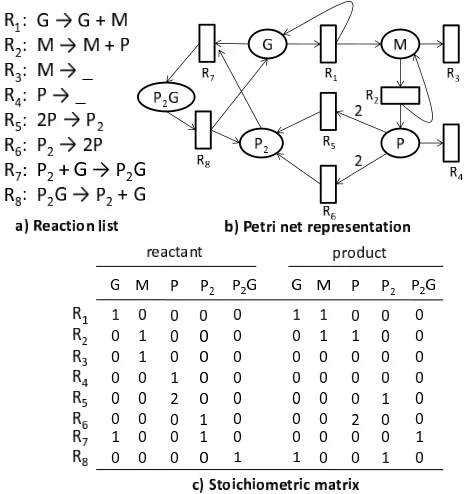
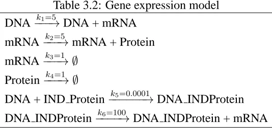
Figure 2.1: The gene expression model is represented by a) a coupled reaction list, b) a Petri-net and c) the corresponding stoichiometric matrix
To store the underlying bipartite graph of a graphical model in a computer, we make use of a matrix. An element in the matrix is corresponding with an di-rected edge between two nodes. The corresponding element is set with a value is the weight (stoichiometry) of such edge. Such matrix is generally referred to as the stoichiometric matrix. Since the matrix is often sparse (with many zero elements), we can apply the sparse matrix computation techniques to re-duce its size and processing time. The figure 2.1 gives an example of different representations for the gene expression model.
2.3
Simulation algorithm
2.3.1 Exact stochastic simulation
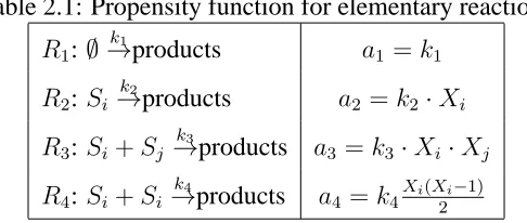
Table 2.1: Propensity function for elementary reactions
R1: ∅
k1
→products a1 =k1 R2: Si
k2
→products a2 =k2·Xi
R3: Si+Sj k3
→products a3 =k3·Xi·Xj
R4: Si+Si k4
→products a4 =k4X
i(Xi−1)
2
speed of molecular species in the cell volume, by these assumptions, become randomized. In fact, they are randomly distributed following the thermodynam-ics law. We therefore only need to consider the population of molecular species, while ignoring all the positions, velocities of species. LetXi(t) denote the
pop-ulation of species Si at time t. Thus, the state vectorX(t) of the system at time
tis represented by a n-vectorX(t) = (X1(t), ..., Xn(t)).
The change of the system state at time t+ dt which is the consequence of the next reaction Rj firing is denoted by a state change vectorvj. Note thatvj is
corresponding to a row of the stoichiometric matrix. Thus, the state transition of the system is formulated as:
X(t+dt) =X(t) +vj (2.2)
The quantity characterizing the probability reaction Rj firing is termed a
propensity function aj. It is defined so that aj(x)dt is the probability reaction
Rj will fire in the next infinitesimal timet+dtgiven the current stateX(t) = x
at timet. This is referred to as the fundamental hypothesis [60] of the stochastic kinetics simulation. A physical derivation for the existence of such propensity function for the elementary reactions is provided in [60, 111]. We summarize the form of these formulas in the following table 2.1.
X(t0) =x0 at timet0 given in Equ. 2.3.
∂P(x, t|x0, t0)
∂t =
m
X
j=1
aj(x−vj)P(x−vj, t|x0, t0)−aj(x)P(x, t|x0, t0)
(2.3) Equ. 2.3 is generally called the chemical master equation (CME). It com-pletely determines the time evolution of the system at any particular time t. CME is indeed a collection of differential equations describing all the state tran-sitions by biochemical reactions. The number of equations in CME is thus in-creasing exponentially with all possible state transitions. For example, let con-sider a system where each species has only two states: 0 and 1. For n species we will have total 2n equations. A full analytic solution of CME is obviously
intractable for most of practical problems wherenis large enough. Some recent computational approaches [116,172] have tried to solve CME directly but at the cost of an approximation error. In this thesis, we exploit the simulation tech-nique to sample the possible solutions of CME instead. The simulation realizes a trajectory of the system evolution by sampling the next reaction probability density functionp(τ, j|x, t), in whichp(τ, j|x, t)dτ is the probability a reaction will be fired in the next timet+τ+dτ and it is the reactionRj, provided that we
are in stateX(t) =x. The next reaction probability is indeed a joint probability of the firing timeτ and the selected probability of reaction Rj. We have:
p(τ, j|x, t)dt= aj(x)exp(−a0(x)τ)dt (2.4)
where
a0(x) =
m
X
j=1
aj(x) (2.5)
time is a discrete probability mass function aj/a0. There are two
implementa-tions of SSA which have the same stochastic behaviour were introduced. They are known as the Direct Method (DM) and the First Reaction Method (FRM).
DM directly computes the reaction firing time τ by inverse the exponential distributiona0exp(−a0(x)τ), and then searches for reactionRj to fire according
to its probabilityaj/a0. DM requires two random number for doing a simulation
step. Let r1 and r2 be random numbers generated from a uniform distribution U(0,1). The first number is used to compute the firing timeτ, while the second one is used to decide which the reaction Rj fires at that time.
τ = 1
a0(x)ln
1
r1
(2.6)
j = the smallest j s.t.
j
X
k=1
ak(x) > r2a0(x) (2.7)
The search for a reaction firing Rj in DM is directly implemented by
con-tinuously accumulating the sum of propensities on-the-fly until it satisfies the condition Pj
k=1ak(x) > r2a0(x). It is equivalent with a linear search.
Having the timeτ and the fired reactionRj, DM jumps current system state
to the new state x+ vj, and updates current time to the new time t+ τ. The
propensities of reactions are updated to reflect the change in the system state as well. The simulation will loop until the current time is passed over a predeter-mined simulation timeTmax. We briefly outline the DM algorithm in Alg. 1 for
the ease of reference.
The key point of the DM algorithm is the propensities aj(x)s are computed
once at the start of the simulation, and then updated as soon as the state x
Algorithm 1 Direct Method (DM)
1: initialize system timet= 0and system statex=x0
2: whilet < tmaxdo
3: for all reactionRj do
4: computeaj
5: end for
6: computea0
7: generate two random numbersr1, r2 ∼U(0,1)
8: setτ = 1/a0(x)ln
1
r1
9: search for the next reaction Rj by continuously accumulating propensities aj until
Pj
k=1ak(x)> r2a0(x)
10: update the timet=t+τ and system statex=x+vj
11: end while
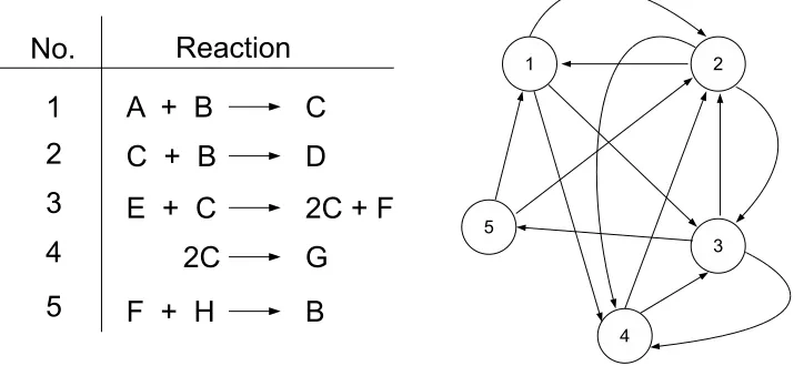
have to be recalculated their propensities. The dependency graphDG(V, E)is a directed graph (see Fig. 2.2 for an example) which contains the reactions as ver-tices V, while an directed edge e(Ri, Rj) ∈ E if and only if Rj ∈ affects(Ri),
the set of reactions affected byRi. Formally
affects(Ri) = {Rj |(reactants(Ri)∪products(Ri))∩ reactants(Rj) 6= ∅} (2.8)
where reactants(Ri) and products(Ri) are the set of species taking part in
reac-tion Ri as reactants and products, respectively. Because a directed catalyst is
not consumed by the reaction itself, it is excluded from the reactants and prod-ucts of the reaction. Hence, by the dependency graph update mechanism, the propensity updates are now reduced to be model-dependent.
FRM is mathematically equivalent with DM but proceeds in a different man-ner. It is a type of racing algorithm. The reaction with smallest putative time is selected to fire next. Thus, in each simulation loop, m random numbers
r1. . . rm ∼ U(0,1) are used to generate the putative times of reactions. The
putative timeτj of reactionRj is computed as:
τj =
1
aj(x)
ln
1
rj
Figure 2.2: Dependency graph (removing self affected edges)
The reaction Rj having the smallest putative time τj = min(τ1, . . . , τm) is
se-lected to fire. The propensity update in FRM is done similar to DM. The mathe-matical equivalence between FRM and DM is derived directly from the property of the exponential distribution [60].
notable improvement of FRM as a discrete-event simulation is the Next Reac-tion Method (NRM) [59]. NRM uses a special priority queue, called the binary heap, to store the putative reaction times. Retrieving the smallest putative time is constant since it is always on the top of the heap. After a reaction is selected to fire, NRM has to maintain the priority queue to reflect the change in the sys-tem; however, it does this in a clever way. NRM exploits the scaling properties of the exponential distribution and dependency graph to improve the propen-sity updates. By this way, the absolute putative time has to be used, instead of relative putative time in original FRM. There are two cases the computing of new putative times and maintaining the heap are required. In the first case, the reaction that has to update its propensity is itself the reaction firing. The new reaction propensity is evaluated. Then, the new putative time is generated following Eq. 2.9. In the second situation, the reactions are dependent reac-tions (the affected reacreac-tions in the dependency graph). The scaling property of exponential distribution will be exploited to scale up their putative times. As-suming that the system moves from the state x to the new state xnew with the
firing timet. Letτnew
j be the new putative time of reaction Rj at this new state.
It is scaled as τjnew = (aj(xnew)/aj(x))(τj − t) + t. So, we do not need to
generate additional random numbers for updating the putative times of affected reactions. There only one random number is required for each simulation step. This would save a lot of computational resource as the number of reactionsm
is large. In fact, the complexity of a call to binary heap consolidation takes logarithmic time i.e.,O(log(m)). Thus, NRM, in worst case, takes logarithmic time for a simulation loop assuming a constant number of affected reactions in the model.
is exponentially increasing. The reactions in entire network is possibly not able to introduce to the simulation at beginning. Moleculizer takes over this problem by introducing the species and reactions to the simulation only as needed. The propensity of new introduced reactions will be modified in consistency with physical properties of this reaction. The new introduced reaction event is then efficiently controlled by a simplified version of queue-event data structure in NRM.
Although NRM is often faster than FRM, DM, it also exposes challenges for implementing the complex data structure used. In some special classes of problems, the complex data structure even negates the performance of NRM. For example, in [29], it showed that the runtime of NRM is actually slower than DM when applied for highly coupled and multiscale reactions models e.g., the heat shock response model of E. Coli. In [29], it also introduces an formu-lation to improve the performance of DM. This new formuformu-lation is called the Optimized Direct Method (ODM). ODM improves the search of DM based on a careful observation that the searching of the next reaction firing will faster if propensities are sorted in descending order. Indeed, the constraint in Eq. 2.7 is faster to satisfy if we rearrange the propensities in a descending order. This new formulation will achieve a great speed up gain if the system contains dis-parate ranges of propensity values. In ODM, the order of propensity values is predicted by pre-run simulations. The average values of propensities are used as criteria for ordering the reactions. The Sorting Direct Method (SDM) [110] shares the same idea with ODM, but it uses a different technique to order the reactions. SDM dynamically bubbles the reactions instead. Anytime a reaction fires, its new propensity is computed. Its index is then exchanged with the next lowest propensity (if exists). The bubble step is also applied to all affected re-actions. At the end, an order for reactions propensities is established without a pre-run simulation.
It, however, potentially makes the search less accurate [65]. A truncation error can happen when the sum of the biggest propensities is represented by a fixed-size floating number. For example, consider a floating point number with k
precision in a computer representation. If the propensity of a reaction is k or-ders of magnitude smaller than the sum of biggest propensities placed before it in the decreasing sorted order. This reaction is thus never selected to fire if a decreasing order of propensity values is used. The implementation of sorting of reaction should require an infinite precision number representation. However, the most restriction of linear search, even reactions are ordered, is its time com-plexity, in the worst case, is increasing linearly with the number of reactionsm, i.e.,O(m). The search thus becomes very slow to as applied to large models.
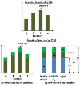
There are several formulations have been proposed during time to reduce the complexity of the linear search used in DM. One possible approach is divid-ing the reactions into groups. The search is now composdivid-ing of two consecu-tive steps. First, the group containing the next reaction is discovered. Second, the next reaction firing in the corresponding group is retrieved out. In [106], these two steps are done through two linear searches. The first search discov-ers the group based on the total propensity of each group. And, the second search retrieves the next reaction firing in corresponding group by its propen-sity. In [145, 147], the grouping of reactions is also exploited, but the search of the next reaction in group is implemented by an acceptance-rejection pro-cedure. A group is associated with a constraint. More precisely, reaction Rj
belonging to group k must satisfy the group constraint: bk−1 ≤ aj ≤ bk where
b is a selected base (e.g., b = 2 in [147]). Then, the search of reaction firing is done as follows. A standard linear search is conducted to find out a group
constant time. The assumptions for the constant time of CR-SSA are: 1) the number of dependent reactions of a firing reaction should be restricted to a con-stant factor, and 2) the reaction propensities which are varied by reaction firings are less significant. Once these assumptions are violated, CR-SSA will spend a lot of time adding and removing reactions to appropriate groups. The CR-SSA performance therefore can be very slow. This has been shown by experiments in [106].
If reactions are divided into groups so that each group contains only two reactions, the search of the next reaction thus needs only one comparison to discover the next branch in the search path. In this sense we have a binary search [18, 103, 156]. The binary search obviously achieves better performance than linear search, but it requires to pre-compute the partial sums of propen-sities. These values have to be stored in a tree structure so that we can apply the dependency-graph update mechanism. The time complexity of a tree-based search SSA is logarithmic both in search and update. We are going to the detail of the tree-based search on the next chapter. There we also predict and discuss the tree leading to the optimal search length.
A different approach to improve SSA is discussed in [141]. It exploits the
uniformization technique to improve the simulation performance. The idea of
uniformization technique is using the upper-bound of total propensity to dis-cretize the time. By the application of the upper-bound of total propensity, this approach introduces a dummy reaction, without changing the system state, to the current set of reactions. The rate of the dummy reaction is equal to the dif-ferent between the upper-bound value and the current total propensity. Because the firing time of all reactions, including the dummy reaction, is all exponential distributed with the same mean corresponding to the inverse of the total propen-sity upper-bound, we do not need to generate the reaction firing time. Only the search of reactions and propensity updates are required. in order to approxi-mate the upper-bound of total propensity it has to know a global upper-bound for the population of all species. This is hard to pre-compute. Indeed, even in the case such upper-bound is known, it may be several orders of magnitude larger than the actual total propensity e.g. if the system is stiff. In this case, sim-ulation would spend a lot of time firing the dummy reaction, hence frequently following self-loops.
2.3.2 Approximate stochastic simulation
Essentially, an approximate method speeds up the simulation by sacrificing its accuracy. It tries to execute as many as possible the number of reaction events in one simulation step. This is the main different with SSA where only one reaction event occurs at time. There are many approximate methods introduced, see for example [62, 115, 134], in which the most notable algorithm is the τ -leaping method. The time axis inτ-leaping is divided into (small) time intervals. The changes of all reaction propensities in a time interval are considered less significant and assumed to be constant. This condition is known as the leap
condition.
reaction Rj satisfies the leap condition. In other words, the propensityaj(x) is
remained essentially constant during that time interval. The number of times reaction Rj occurring is so a Poisson process P oisson(aj(x)τ). Let kj be the
number of times reaction Rj fires during the time interval [t, t+ τ). Thus, we
have that kj ∼ P oisson(aj(x)τ). Each occurrence of Rj causes the system
state to change an amount x + vj. So, the net change of the system state by
firingkj times reaction Rj in the time interval [t, t+τ) isx+kj ·vj. Based on
this observation the τ-leaping is proceeding as follows.
The simulation time Tmaxis divided into time intervals [t, t+τ)so that the
leap condition is satisfied on each interval. In each simulation step, m Poisson random numbers kj ∼ P oisson(aj(x)τ)for all j = 1. . . mare generated. The
system state changing by mreactions firing in an interval are updated by:
X(t+τ) = X(t) +
m
X
j=1
kjvj (2.10)
The accuracy of theτ-leaping thus is strongly depending on the choosing of an appropriate τ value. In principle, a post-leap check can be applied. That is we start with an predefined arbitrary (small) τ value. Then, we check the difference in the reaction propensity after that leaf. If all the differences are acceptable (i.e., satisfying the leap condition) then the leaf is accepted. Oth-erwise, τ should be reduced. More precisely, let x and xτ be the state before and after the leap τ. The absolute change in propensity of reaction Rj is
com-puted and ensured to be sufficiently small comparing with an error parameter ǫ, i.e., kaj(xτ)−aj(x)k < ǫ for all j = 1. . . m. If the change in propensity of
any reaction violates this condition,τ is reduced e.g., to a half, and the checking procedure repeats. The post-leap working in this manner, however, potentially biases the system away from large yet reasonable changes in the state.
whether it is acceptably small. Several strategies have been introduced for doing the pre-leap check. In [62] the expected change in propensities is suggested to be bound by a0(x), i.e., kaj(xτ)−aj(x)k ≤ ǫa0(x) for all j = 1. . . m where
0< ǫ ≪1is the error control parameter. This original idea of the leap selection is extended and improved by [26, 66]. In [27], a new leap selection procedure is proposed in which the relative change in propensity of a reaction is bound by its current propensity instead of total sum of propensities.
A subtle problem occurring in the τ-leaping is the negative population of species. The Poison random variable kj ∼ P(aj(x)τ), in general, is unbound.
The population of a species after the leap thus can get negative. It is obviously unrealistic and should be prevented during the simulation. Several solutions have been introduced to solve the negative population. In [32, 159] a Binomial distribution with the same mean with the Poison process P(aj(x)τ) is used
In [11] the K-leap method and in [22] the R-leap method, respectively, are alternatives for the τ-leaping method. The advantage of these methods is the number of reaction firings during a leap is controllable. The negative popula-tion never happens, and thus improving the simulapopula-tion accuracy. These meth-ods are variants of kα-leaping method proposed in [62]. The principle of these
methods is the total number of reaction firings during a leap is predefined and constrained. The leap τ is proved to be following a Gamma distribution, while the number of times a reaction firings during a leap is following a Multinomial distribution. Then, several sampling techniques have introduced for both of these methods to generate a suitable τ value.
Theτ-leaping is not only used for improving the performance of SSA, it but also bridges a connection to the deterministic simulation [65]. Let suppose the leap condition is relaxed so that τ is still small enough to satisfy the leap condi-tion, but the expected number of reaction firings in a leap is also large enough, i.e., aj(x)τ ≫ 1 for all j = 1. . . m. By this new condition, the Poisson
dis-tribution is approximated by a Normal disdis-tribution with the mean and variance are aj(x)τ. Thus, Eq. 2.10 is rewritten by:
X(t+τ) = X(t) +
m
X
j=1
Nj(ajτ, ajτ)vj
= X(t) +
m
X
j=1
vjajτ + m
X
j=1
vj√ajNj(0,1)√τ (2.11)
where Nj(µ, σ2) denotes a Normal distribution with mean µ and variance σ2.
To derivation of Eq 2.11 makes use a special property in conversion of a Nor-mal distribution to standard NorNor-mal distribution N(0,1) i.e., Nj(µ, σ2) = µ+
σN(0,1).
dX(t)
dt =
m
X
j=1
vjaj + m
X
j=1
vj√ajΓj(t) (2.12)
whereΓj(t) is an independent Gaussian white-noise process.
In the thermodynamic limit, where the volume size and the species popu-lation is increasing to infinity, but the species concentration (the ratio between species population and volume size) is kept roughly constant, the random fluctu-ation termPm
j=1vj√ajΓj(t) in Eq. 2.12 grows slowly (in square root)
compar-ing with other terms (in linearity). This term is thus negligible small contribute to the macroscopic change of the system and can be ignored. In other words, the fluctuation in population of species in Eq. 2.12 is able to remove. Eq. 2.12 approximate to be:
d[X]
dt =
m
X
j=1
f([X]) (2.13)
in which[X]denotes the species concentration vector, and a functionf presents the changes of the species concentration by reactions. The Equation 2.13 is the general form of RREs used in deterministic simulation. Hence, the stochastic approach in the thermodynamic limit converges to the deterministic one.
2.3.3 Hybrid stochastic simulation
The principle of the hybrid approach is dividing the system into two sub-systems. These parts will be simulated by different simulation methods, but they are complementary to each others. An intuitive partitioning strategy is to partition reactions into subsets of fast and slow reactions. Mathematically, it is equivalent to partition CME. The fast reactions often, but not always, involves high population species. The rest will be called slow reactions. Two subsys-tems are assumed to evolve independently. The fast reactions is integrated by, e.g., an ODE solver. The slow reactions is simulated by an SSA variant to retain the important fluctuations. Because the slow reactions, in general, is dependent to the fast species, their propensities can change if a fast reaction fires. For this reason, the propensity of slow reaction have to modify to use the random time varying propensity.
For the success of a hybrid method, several aspects have to be considered. First, the criteria as well as their reliability are applied for partitioning of the system. Second, how the partition is done in static or in dynamic. Third, how the synchronization between simulation techniques i.e., between the determin-istic vs. stochastic as well as the data conversion i.e., between the species con-centration vs. population, continuous vs. discrete. Lastly, how to treat the fast reactions involving also the low population species.
There are several hybrid methods has been proposed in literature. We review three main approaches in the following.
is no slow reaction event occurring. The time-varying propensities of the slow reactions in this time step are evaluated. Then, the firing timeδtfor a slow reaction event is derived. In particular case, the time step∆tis chosen small enough so that the changes in slow reaction propensities are assumed to be constant. The computing of the slow reaction event thus does not require to use the random time change technique and is greatly simplified. Finally, the simulation decides which event will update the system. If the slow reaction event is occurring before the ODE integration, i.e.,δt < ∆t, a slow reaction is fired. The fast species involved in this slow reaction is updated as well. In the other case, only the ODE integration takes place. A new simulation iteration is executed after that.
• The CLE/SSA hybrid. This hybrid simulation is a combination of a dis-crete simulation for slow reactions and a CLE solver for fast reactions [72, 140]. The partitioning of reactions is treated dynamically. A reaction is considered to be fast if it satisfies the conditions 1) aj∆t ≥ λ and 2)
x ≥ ǫ|vj| in which ∆t is the time step for updating the fast reactions, λ
and ǫare parameters to control the partitioning. For example, in [140], λ
and ǫare assigned to be 10 and 100, respectively. During the time course if a fast reaction violates the partitioning condition, it is automatically moved to slow reaction subset. The CLE/SSA achieves higher accuracy than ODE/SSA because it still could capture for the fluctuations in the fast reactions.
• Theτ-leaping/SSA hybrid. Theτ-leaping/SSA hybrid places in the middle between deterministic and stochastic hybrid. It is named as the maximal
above. However, by applying a variant of τ-leaping for the fast subset makes this hybrid approach become more difficult to analyze the time-varying nature of slow reaction propensities. Thus, this technique puts an assumption that the changes in slow reaction propensities during a leap is less significant, and is ignored. This, of course, introduces an additional source of error to the simulation.
2.3.4 Stiff system simulation
The stiffness arises in systems consisting both fast and slow reactions where the fast reactions approach the stable state very fast. After rapidly transient time with a very short fluctuation due to fast reactions, the system becomes stable. The slow reactions then determine the system dynamics. The presence of multiple time scales in such system slows down the stochastic simulation significantly. In fact, SSA spends most of its simulation time for simulating fast reaction events; however, this is not corresponding to the system dynamics.
Many methods have been proposed for efficiently simulating the stiff sys-tems. They are often based on two main techniques: the quasi-steady state as-sumption (QSSA) and the partial equilibrium asas-sumption (PEA), which are used in the deterministic context and adapted to the stochastic simulation. The QSSA improves the simulation performance by removing intermediate and highly re-active species from the model, while PEA enhances the simulation by assuming fast reactions reaching equilibrium will remain always in that equilibrium state. The difference between QSSA and PEA is the object they focus on. The for-mer focuses on the state, while the latter concentrates on the reactions. In the following we briefly review these techniques.
other words, two following assumptions are made. First, the probability distri-bution of intermediate species z conditional on y approximatively satisfies the definition of the CME. That is P(z|y, t) follows the form of chemical master equation in eq. 2.3. Second, the net rate of change for the conditional probabil-ity distribution of these intermediate species is approximatively equal to zero. It is equivalent that dP(z|y, t)/dt ≈ 0. By these two assumptions, the stationary probability distribution of intermediate speciesP(z|y) is more easier to derive. An analytic solution or a numerical computation can be conducted to sample the population of intermediate species. Having the knowledge of intermediate species, reaction propensities involving the primary speciesy for doing stochas-tic simulation become easier to derive. In fact, these propensities have the form
bk(y) =
P
zak(y, z)P(z|y).
Summing up, in each QSSA-based simulation loop two consecutive steps are done. First, the intermediate speciesz is sampled from the stationary distri-butionP(z|y). They are substituted into the computation of propensitiesbk(y)
involving primary species. And second, a SSA step is applied to find the next reaction firing based on propensitiesbk(y). Note that when a reaction firing only
the population of primary speciesy is updated.
The PEA-based stochastic simulation. The slow-scale SSA (ssSSA) [23, 24] is an example of PEA. ssSSA proceeds as follows. It provisionally divides reactions into fast reactions, denoted Rf, and slow reactions, denoted Rs. The
provisionally partitioning of reactions is decided only by their rate constants. The fast reactions are further assumed to remain always in equilibrium state upon reaching the equilibrium. Species whose population gets changed by a fast reaction are labeled as fast speciesSf, the rest species is called slow species
Ss. By this definition, a fast species clearly can change by a slow reaction,
but the reverse direction is not true. The corresponding process X(t) is thus divided into a fast process Xf(t) and Xs(t). Although the full state vector
overcomes this difficulty by introducing the definition of virtual fast process. More precisely, the virtual fast processX˜f contains the same species as the fast
species Xf(t) where all slow reactions turned off. Thus, the virtual fast process
˜
Xf only depends on fast species, while the slow species are assumed constant. The P˜(Xf, t) in this definition is completely described by CME.
The virtual process X˜f, under the stiffness property, is assumed to be a sta-ble process. It thus imposes two assumptions. First, the stationary distribution
˜
P(xf,∞) exists. Second, the relaxation time of X˜(t) to stationary asymptotic
form, X˜(t) → X˜(∞) happens very quickly (typically, smaller than the time to the next slow reaction event). With these two assumptions, the stationary distri-bution P˜(xf,∞)is analytically solvable by e.g. a numerical method. Thus, the
population of fast species involved in the virtual fast process can be computed without doing simulation. The simulation now only applies for slow reactions where the propensity of a slow reaction is adapted as follows. Let∆sbe the time
which is very large compared to relaxation time of X˜f(t), but also very small
compared to the expected time to the next slow reaction. The probability one slow reaction Rsj occurs in interval[t, t+ ∆s)is approximated byasj(xf, xs)∆s
where as
j(xf, xs) is referred to as slow scaled propensity function of reaction
Rs
j. It is given by:
asj(xf, xs) =X
xf′
˜
P(xf′,∞|xf, xs) (2.14) In conclusion, a ssSSA execution for sampling a trajectory is first numer-ically calculating the population of fast species. The fast species are indeed generated by randomly sampling the limited virtual fast processX˜f(∞). Then,
2.3.5 SSA Extensions
Several extensions also have been introduced to cover different aspects of bio-chemical reactions systems by relaxing SSA underlying hypothesis. In this sec-tion we briefly review two such relaxasec-tions that are: the reacsec-tion with delays, and reaction with spatiality.
Reaction with delays. In SSA, the next reaction assumes to happen instan-taneously. Biochemical reactions, in fact, will take a certain time to finish after they are initiated. The delayed time in biochemical reactions is thus inevitable, but it is often many orders smaller than the waiting time to the next reaction. The delayed time is therefore often ignored. The delayed time, however, will introduce a another source of noise and plays a crucial role in the development of the biochemical processes if it is in the order of the reaction time. For exam-ple, in [13], the effect of delayed time to the development of the gene expression has been observed. The system exhibits the stochasticity even the counterpart is deterministic. The delayed-time reactions could further use to reduce the deleterious effects of propagation noise.
reaction is discarded and the update of the delayed reaction is performed. An exact generalization of SSA covering all possible delays in reactions, called the delay stochastic simulation algorithm (DSSA), is introduced in [21]. An effi-cient modified of NRM for the delayed time reactions is also introduced recently in [6].
Reaction with spatiality. This extension considers relaxing the well-mixed assumption. The spatial homogeneous is easy to validate by in vitro experi-ments where the diffusion of molecular species is much faster than the reaction. However, it is in general not true for living cells. The species in cell environ-ment is indeed very highly localized to improve cellular functions. The cell division, metabolic and signaling pathways, for example, strongly depend on the spatial information. The temporal evolution of SSA by reactions alone is not enough to reproduce important effects such as the molecular crowding, the excluded volume effect. It therefore should be extended to take into account the diffusion of species in space.
Several approaches adapted SSA to make it applicable for simulating the diffusion of species in space. The key idea of these extensions is diving the space into smaller subvolumes. The subvolume size length is chosen to be small enough so that the well-mixed assumption inside that subvolume is satisfied. SSA therefore can be applied to simulate reactions inside a subvolume. The diffusion of a species between subvolume is treated directly as a unimolecular reaction. The rate of diffusion is translated from the bulk diffusion by the Fick’s law. The rate of the diffusion reaction, in general, should depend on the shape of subvolume. The modelling of the spatial information in such the way is often referred to as reaction-diffusion master equation (RDME). RDME is indeed a natural extension of CME for spatial heterogeneous.
biochem-ical reaction, the population of reactants involved in that reaction is updated. Then, only affected reactions in the current subvolume have to update propen-sities. In case the selection is a diffusion reaction, the diffusive species selects a random neighbor to move to and the population of this species in these sub-volumes is updated. For anisotropy diffusion, the destination subvolume of a diffusive species should be explicitly defined instead of random selecting a neighbor. The affected reactions due to the diffusive species in both of these subvolumes update their propensities after that. The direct application of SSA for doing reaction-diffusion simulation, however, is often computation and/or memory inefficient. A possible improvement is dividing the selection of the reaction firing into two consecutive search steps. The first search discovers the subvolume containing the next reaction firing, then the second one retrieves out the next reaction firing within that subvolume. There are many possible combi-nations for doing these steps, e.g., two consecutive DMs. The next subvolume method (NSM) [45] is a notable formulation of spatial SSA extension in this way for sampling RDME. NSM is indeed a clever combination of NRM and DM. In NSM, the selection of the next subvolume using the idea of NRM. The putative times of subvolumes is precomputed and stored in an indexed priority queue. Since the smallest putative time is always on the top of the queue, the selection of the subvolume is in constant time. The next reaction firing in this subvolume will be found out by DM. After the next reaction firing is defined, the population of species and affected reaction propensities in subvolume(s) are updated depending on the type of the selected reaction. Then, the putative times of subvolume(s) are recalculated to reflect the changes. The priority heap of subvolume putative times is consolidated as well. By using the priority queue to select a subvolume, the time complexity of NSM is scaled logarithmic with the number of subvolumes.
the reactions and diffusions are treated separately. The theory behinds GMP is known as the operator splitting technique [35, 36]. In essential, GMP pre-computes the diffusion time of a molecular species based on its diffusion con-stant and the subvolume size length. The time-axis is thus divided into small chunks of the diffusion times. During the simulation, if a diffusion event occurs, the corresponding species in a subvolume is distributed all over its neighbors. Between two diffusion events, reactions between specie