Vol. 14, No. 1, 2017, 161-172
ISSN: 2279-087X (P), 2279-0888(online) Published on 8 August 2017
www.researchmathsci.org
DOI: http://dx.doi.org/10.22457/apam.v14n1a19
161
Annals of
A Fuzzy Programming Approach to Multi-objective
Mean Variance Model
Sahidul Islam1 and Rahul Chaudhury2
Department of Mathematics, University of Kalyani, Kalyani – 741235 West Bengal, India.
1
email: [email protected] 2
Corresponding author. Email: [email protected]
Received 2 July 2017; accepted 26 July 2017
Abstract. The traditional single objective mean variance optimization model fails to
satisfy the investors with multiple investment objectives. So multi-objective portfolio optimization model is considered in this paper. Since this will help investors to achieve highest expected return among the different financial products of the capital market and to fulfill the expected return objectives simultaneously. Fuzzy Non-Linear Programming (FNLP) and Fuzzy Additive Goal Programming (FAGP) techniques are used to solve this multi-objective model. Since it will fulfill the wanted aspiration level of the investors concerning return and risk objectives. And finally solution procedure is illustrated by numerical examples.
Keywords: Multi-objective, Portfolio, Mean-Variance AMS Mathematics Subject Classification (2010): 90C29
1. Introduction
In financial management one of the most important topics is portfolio management. Basically portfolio management gives the direction to obtain a portfolio that will satisfy an investor concerning his risk and return. The main aim of portfolio management is to choose the best amalgamation of assets that will provide the highest expected return while maintaining acceptable level of risk simultaneously.
162
portfolio framework, Markowitz trade-off between expected return and risk of the portfolio , each of them represented by the mean of historical performances i.e. mean of return of an asset and the dispersion of the return as risk respectively.
Over the last few decades the pioneer model proposed by Markowitz, mathematical programming techniques have become necessary tools to support financial decision making process and applied a lot in real life situation. There are several mathematical tools used in general to find the best solution in portfolio optimization. Such as Forecasting, Simulation, Statistical Model, Mathematical programming models. Among these models mathematical programming is the best option to the decision maker to find the optimal solution.
Also several exact method based techniques had been applied to solve the portfolio optimization models, such as integer programming method [1], goal programming method [2], lexicographic goal programming approach [3] etc. Some meta-heuristics based approaches are also used such as simulated annealing [4], genetic algorithm [5], particle swarm optimization [6], ant colony optimization [7]. In [20] authors had discussed about some advanced optimization techniques.
But in practice in order to take best portfolio decisions, decision maker will have to take help of some vaguely define financial parameters such as return more than 20%,
risk lower than 10% etc. Under such vague expression it is difficult to construct
satisfactory portfolios using crisp or interval numbers. In such a situation decision maker has to take help of fuzzy set theory in order to formulate the models of portfolio selection. Not only the uncertainty and the vagueness are controlled by fuzzy set theory, but also help decision maker to take flexible decision by considering the investors’ preferences.
The concept of fuzzy decision theory was developed by Bellmann and Zadeh [8] based on the idea of fuzzy sets introduced by Zadeh in 1965 [9]. Also some authors [10,11,12,13,14] had already used the fuzzy frame work to select the efficient portfolio using mean-variance model. Wang et all [15] had used fuzzy decision theory in single objective portfolio optimization model.
In [22] authors had used a fuzzy programming technique to solve his transportation model. Also Jebaseeli and Dhayabaran had presented a comperative study on fully time-cost trade off.
163
Numerical examples are given to illustrate the problems and then the result will be compared.
2. Mathematical model
The problem of portfolio optimization is to allocate capital over a number of available assets. In portfolio optimization investors hope to achieve maximum portfolio return as well as minimum portfolio risk. Because return is compensated by using risk, it is crucial for the investors to balance the risk return trade off for their investments.
So bi-objective Mean- Variance (MV) model for portfolio optimization considered in this paper based on the mean – variance framework proposed by Markowitz [16] is as follows:
Maximize = ∑ (1)
Minimize = ∑ ∑
Subject to:
= 1,
≥ 0 ,
= 1,2, … … … . , !
where,
is the proportion of the total fund invested in i-th asset, for = 1,2, … … … . . , ! .
"is the random rate of return on the ith asset, for = 1,2, … … … . . , !.
is the expected rate of return on the ith asset, for = 1,2, … … … . . , !.
is the covariance between ith and jth asset return i.e. " and " , for , # = 1,2, … … … . . , !.
$ is the variance of ith asset, for = 1,2, … … … . . , !.
3. Mathematical analysis
In this section we will discuss about fuzzy programming techniques considered in this paper to solve a Multi-Objective Non-Linear Programming (MONLP) problem.
3.1. Multi-objective non linear programming (MONLP) problem
A Multi-Objective Non-Linear Programming (MONLP) may be considered in vector minimization problem form as follow:
%!&'( ) = [), )$, … … … , )+]- (2)
164
Fuzzy programming technique is an efficient method to solve a multi-objective programming problem, which was initially showed by Zimmermann [17].
3.2. Fuzzy programming techniques for a MONLP
The following steps are to be followed to solve a MONLP (2).
Step 1: Solve the MONLP as a single objective programming problem considering each of the objectives at a time, ignoring the others. The solutions so obtained are known as ideal solutions.
Step 2: To find the corresponding values for each of the objectives at each solutions derived from previous step. With the values of all objectives at each ideal solution, and the pay-off matrix can be formulated as follows:
) )$ …. )+
)
(
...
)
(
)
(
...
....
.
..
...
...
)
(
...
)
(
)
(
)
(
....
)
(
)
(
...
* 2 1 2 2 * 2 2 1 1 1 2 1 * 1 2 1 k k k k k k kx
w
x
w
x
w
x
w
x
w
x
w
x
w
x
w
x
w
x
x
x
Here , $, … … … . . , +are the ideal solutions of the objectives
), )$, … … … , )+? respectively. So @A = max{)A, )A$, … … , )AC+D} , And
FA = )A∗A
Here FAand @Aare lower and upper bounds of the rth objective function )Afor =
1, … , H.
Step 3: Using aspiration levels of each objective of the MONLP (2) may be written as follows:
Find so as to satisfy
)A ≤I FA = 1,2, … … … , H, ∈ 5 (3) Here objective functions of (2) are considered as fuzzy constraints. This type of fuzzy constraints can be quantified choosing a corresponding membership function
JAC)AD = K
0 )A ≥ @A
=A FA ≤ )A ≤ @A 1 )A ≤ FA
L
(4)
165
Here =A is a strictly monotone decreasing function with respect to )A .
Having elicited the membership functions (as in (4)) JAC)AD for = 1,2, … . . , H, a general aggregation of the form
JMI = JMIJC)D, J$C)$D, , … … … , J+C)+D is introduced.
So a fuzzy multi-objective decision making problem can be defined as
%<&'( JMI (5)
./0#(12 23 ∈ 5
Then fuzzy decision (By Bellman and Zadeh) [8] based on minimum operator (By Zimmermann) [16] the problem (3) will take the form
%<&'( N
./0#(12 23 JAC)AD ≥ N , for = 1,2, … , H (6)
∈ 5 and 0 ≤ N ≤ 1
This is known as Fuzzy Non-Linear Programming problem (FNLP)
And fuzzy decision based on convex operator (Tiwari et al) [18] the problem (3) will take the form
%<&'( ∑+AJAC)AD (7) O/0#(12 23 0 ≤ JAC)AD ≤ 1, for = 1,2, … , H and ∈ 5 This is known as Fuzzy Additive Goal Programming problem (FAGP)
Step 4: Solve (6) and (7) to get the Pareto Optimal solutions.
3.3. Weighted fuzzy non-linear programming (WFNLP)
Concerning the relative importance of each of the objective functions )A, decision maker prefer positive weights P for = 1,2, … , H. These weights in normalized form will be considered by taking ∑ P+ = 1.
Then considering normalized weights, the fuzzy non-linear programming problem (6) becomes
%<&'( N (8)
./0#(12 23 PAJAC)AD ≥ N, for = 1,2, … , H
∈ 5 <!= 0 ≤ N ≤ 1
)ℎ(( P +
A = 1
3.4. Weighted fuzzy additive goal programming (WFAGP)
166
Then considering normalized weights, the fuzzy non-linear programming problem (7) becomes
%<&'( ∑+APAJAC)AD (9) O/0#(12 23 0 ≤ JAC)AD ≤ 1, for = 1,2, … , H
∈ 5
)ℎ(( P +
A = 1
Few basic definitions of Pareto optimal solutions are presented below.
Definition (Complete optimal Solution)
∗is said to be a complete solution to the MONLP (2) if and only if there exists ∗∈ 5
such that )A∗ ≤ )A for = 1,2, … , H and for all ∈ 5.
But if the objective functions of a multi-objective problems are conflicting in nature, then complete solution does not exist in general and so the condition of Pareto optimality concept is need to be considered and it is defined as follows.
Definition (Pareto optimal Solution)
∗is said to be a Pareto solution to the MONLP (2) if and only if there does not exist
another ∈ 5 such that )A∗ ≤ )A for = 1,2, … , H and ) ≠ )∗ for at least one #, # ∈ {1,2, … , H}.
4. Fuzzy programming technique to solve multi-objective mean-variance model (MOMVOM)
According to Vector Minimization Problem (VMP) the model (1) can be formulated as
Minimize = − ∑ (10)
Minimize =
Subject to:
= 1,
≥ 0 ,
= 1,2, … … … . , !
167
Now the upper bounds @, @$ and lower bounds F, F$ are identified, where F≤ ≤
@ and F$≤ ≤ @$.
For simplicity we have considered linear membership function for the objective functions and defined as follows
JC D = T U
V − F0 ≤ F
@− F F≤ ≤ @ 1 ≥ @
L
JCD = T U
V@$− 0 ≥ @$ @$− F$ F$≤ ≤ @$
1 ≥ F$
L
According to step 3, having elicited the above membership functions crisp non-linear problem of (10) is formulated as follows:
Based on FNLP
%<&'( N (11)
./0#(12 23 ≥ F+ N@− F ≤ @$− N@$− F$
= 1,
0 ≤ N ≤ 1
≥ 0 , = 1,2, … … … . , !
Based on weighted FNLP (WFNLP)
%<&'( N (12)
./0#(12 23 ≥ F+PN
@− F ≤ @$−PN
$@$− F$
= 1,
0 ≤ N ≤ 1 P+ P$= 1
≥ 0 , = 1,2, … … … . , !
Based on FAGP
%<&'( X?YZ\ [
[YZ[ +
\]Y^?
168
0 ≤ − F@ − F ≤ 1 0 ≤@@$−
$− F$ ≤ 1
= 1,
≥ 0 , = 1,2, … … … . , !
Based on weighted FAGP (WFAGP)
%<&'( P_X?YZ\ [
[YZ[` + P$_
\]Y^?
\]YZ] ` (14)
0 ≤ − F@ − F ≤ 1 0 ≤@@$−
$− F$ ≤ 1 ∑ = 1,P+ P$= 1 ≥ 0 , = 1,2, … … … . , !
Solving (11), (12), (13), (14) we will get the Pareto optimal solution to the corresponding problem.
5. Numerical illustration
The model is validated using a data set of 10 randomly selected assets taken from [19] which was actually taken from National Stock Exchange (NSE).
Table 1:
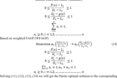
Now the historical return for the entire period is computed which is given in the table below.
Company 1 2 3 4 5 6 7 8 9 10 11 12
169 Table 2:
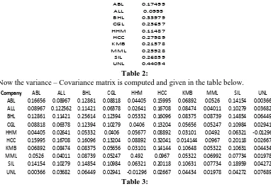
Now the variance – Covariance matrix is computed and given in the table below.
Table 3:
The Pareto optimal solution for the problem (11) by FNLP is given in Table 4.
Table 4:
The Pareto optimal solution for the problem (13) by FAGP is given in Table 5.
Table 5:
The Pareto optimal solution for the problem (12) obtained by WFNLP for different weights are given in the table below:
Table 6:
Company Return
ABL 0.17499
ALL 0.0995
BHL 0.33979
CGL 0.23657
HHM 0.11487
HCC 0.27989
KMB 0.21578
MML 0.25928
SIL 0.26859
UNL 0.44054
Company ABL ALL BHL CGL HHM HCC KMB MML SIL UNL
ABL 0.16656 0.08967 0.12861 0.08818 0.04405 0.15995 0.06892 0.0526 0.14154 0.00366 ALL 0.08967 0.122562 0.11421 0.06378 0.02641 0.16708 0.08474 0.04011 0.10279 0.03682 BHL 0.12861 0.11421 0.25614 0.12394 0.05332 0.16096 0.08375 0.08739 0.14854 0.06449 CGL 0.08818 0.06378 0.12394 0.10279 0.0406 0.13204 0.05656 0.05247 0.10984 0.02941 HHM 0.04405 0.02641 0.05332 0.0406 0.05677 0.08892 0.03101 0.0492 0.06321 -0.01296 HCC 0.15995 0.16708 0.16096 0.13204 0.08892 0.32041 0.014144 0.0967 0.20118 0.02667 KMB 0.06892 0.08474 0.08375 0.05656 0.03101 0.14144 0.10648 0.05322 0.10631 0.04434 MML 0.0526 0.04011 0.08739 0.05247 0.492 0.0967 0.05322 0.06992 0.07734 0.01978 SIL 0.14154 0.10279 0.14854 0.10984 0.06321 0.20118 0.10631 0.07734 0.18959 0.04272 UNL 0.00366 0.03682 0.06449 0.02941 -0.01296 0.02667 0.04434 0.01978 0.04272 0.07689
ABL ALL BHL CGL HHM HCC KMB MML SIL UNL Return f(x) Risk g(x)
0 0 0 0 0 0 0 0.1100412 0 0.8899576 0.420594 0.902066486
0 0 0 0 0.1012954 0 0 0.09825821 0 0.8004404 0.389738 0.830304144
0.0004173 0 0 0 0.2811498 0 0 0 0 0.7184266 0.348864 0.797584608
0.000266 0 0 0 0.4298791 0 0 0 0 0.5698523 0.300469 0.754761207 Weights
weight for f(x) =0.2, weight for g(x)=0.8
Weight for f(x) =0.4, weight for g(x)=0.6
weight for f(x)=0.6, weight for g(x)=0.4,
170
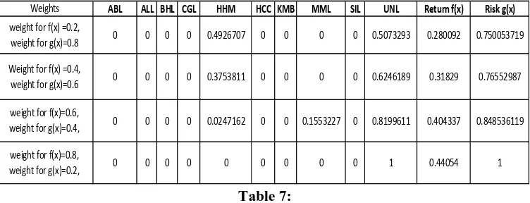
The Pareto optimal solution for the problem (14) obtained by WFAGP for different weights are given in the Table 7.
The Pareto optimal solution for the MOMVOM by FNLP and FAGP is given the table 4 and 5 respectively, where as the solution by WFNLP and WFAGP is given in table 6 and 7 respectively. Here, FNLP method gives more return whereas FAGP method gives less risk. So FAGP method gives better results for risk and FNLP method gives better results for return. After incorporation of weight from WFNLP we have, while increasing the weight associated with the return objective function the return obtained gradually decreases while from WFAGP the return associated with greater weight to the return objective function gradually increases. The opposite situation occurs for risk objective function. From WFNLP we have, while increasing the weight associated with the risk objective function the risk obtained increases, whereas from WFAGP while increasing the weight associated with the risk objective function the risk obtained decreases.
Table 7:
And lastly from the above solution tables obtained by FNLP and FAGP we conclude that in weighted FNLP method weight may be effect on directly to the objective functions but in the weighted FAGP method weight may be effect on inversely to the objective function.
5. Conclusion
In this paper, we had considered Bi-objective Mean- Variance model for portfolio selection. Two fuzzy non-linear programming techniques based on FNLP and FAGP are used to solve the model. Also weights are considered on both the objective functions and then the models are solved by WFNLP and WFAGP method. From the result it is clear that fuzzy non-linear programming technique is an efficient technique and may be used in any other financial optimization model.
Acknowledgement. The authors are thankful to Department of Mathematics, University
of Kalyani for providing financial assistance through DST-PURSE program and UGC-SAP program. Also the authors are thankful to the referee for their valuable suggestions.
ABL ALL BHL CGL HHM HCC KMB MML SIL UNL Return f(x) Risk g(x)
0 0 0 0 0.4926707 0 0 0 0 0.5073293 0.280092 0.750053719
0 0 0 0 0.3753811 0 0 0 0 0.6246189 0.31829 0.76552987
0 0 0 0 0.0247162 0 0 0.1553227 0 0.8199611 0.404337 0.848536119
0 0 0 0 0 0 0 0 0 1 0.44054 1
Weights
weight for f(x) =0.2, weight for g(x)=0.8
Weight for f(x) =0.4, weight for g(x)=0.6
weight for f(x)=0.6, weight for g(x)=0.4,
171 REFERENCES
1. P.Bonami and M.A.Lejeune, An exact solution approach for portfolio optimization problems under stochastic and integer constraints, Operations Research, 57(3) (2009) 650-670.
2. K.Pendaraki, C.Zopounidis and M.Doumpos, On the construction of mutual fund portfolios: A multicriteria methodology and an application to the Greek market of equity mutual funds, European Journal of Operational Research, 163(2) (2005) 462-481.
3. H.P.Sharma and D.K.Sharma, A multi-objective decision-making approach for mutual fund portfolio, Journal of Business and Economics Research, 4(6) (2006) 13-24.
4. Y.Crama and M.Schyns, Simulated annealing for complex portfolio selection problems, European Journal of Operational Research, 150(3) (2003) 546 – 571. 5. H.Zhu,Y.Wang, K.Wang and Y.Chen, Particle Swarm Optimization (PSO) for the
constrained portfolio optimization problem, Expert Systems with Applications, 38(8) (2011) 10161-10169.
6. T.Cura, Particle swarm optimization approach to portfolio optimization, Nonlinear
Analysis: Real World Applications, 10(4) (2009) 2396-2406.
7. G.F.Deng and W.T.Lin, Ant Colony Optimization for Markowitz Mean-Variance
Portfolio Model, Swarm, Evolutionary, and Memetic Computing, Springer Berlin
Heidelberg, (2010) 238-245 .
8. R.E.Bellman,. and L.A.Zadeh, Decision making in fuzzy environment, Management
Sciences, 17(4) (1970) 141-164.
9. L.A.Zadeh, Fuzzy Sets, Information and Control, 8 (1965) 338-353.
10. A.B.-Terol, B.P.-Gladish, M.A.-Parra and M.R.Yrfa, Fuzzy compromise programming for portfolio selection, Applied Mathematics and Computation, 173 (2006) 251-264.
11. S.Ramaswamy, Portfolio selection using Fuzzy decision theory, Bank of
International Settelement working papers No 59 , Monetary and Finance Department,
Basle (1998).
12. M.A.Parra, A.B.Terol and M.V.R.Uria, A fuzzy goal programming approach to portfolio selection, European Journal of Operation Research, 133 (2001) 287-297. 13. J.Watada, Fuzzy portfolio selection and its application to decision making, Tatra
Mountains Mathematical Publications, 13 (1997) 219-248.
14. W.Zhang and Z.Nie, On admissible efficient portfolio selection problem, Applied
Mathematics and Computation, 159 (2004) 357-371.
15. S.Y.Wang and S.S.Zhu, Fuzzy portfolio optimization, International Journal of
Mathematical Science, 2 (2003) 133-144.
172
17. H.J.Zimmermann, Fuzzy programming and linear programming with several objective functions, Fuzzy Sets and System, 1 (1978) 45-55.
18. R.N.Tiwari, S.Dharmar and J.R..Rao, Fuzzy goal programming: An additive model,
Fuzzy Sets and System, 24 (1987) 27-34.
19. Fuzzy Optimization in Portfolio- Advances in Hybrid Multi-criteria Methodologies,
Studies in Fuzziness and Soft computing, Springer, Vol. 36.
20. D.K.Biswas and S.C.Panja, Advanced Optimization Technique, Annals of Pure and
Applied Mathematics, 5(1) (2013) 82-89.
21. S.Goswami, A.Panda and C.B.Das, Multi-objective cost varying transportation problem using fuzzy programming, Annals of Pure and Applied Mathematics, 7(1) (2014) 47-52.