Implementation Technique and Analysis of Power Flow in AC Transmission Circuits

Implementation Technique and Analysis of

Power Flow in AC Transmission Circuits

M. C. Anumaka

Department of Electrical/Electronic Engineering, Faculty of Engineering, Imo State University, Owerri, Nigeria

Abstract

The power flow analysis and its implementation in AC transmission network have become indispensible in a wide range of power system planning and operation. This paper focuses on the theory and algorithms of power flow analysis, which is essential to the understanding of the methodology of modern power flow analysis. The study gives explicit explanation of the fundamentals of power flow study and solution formulation, emphasized the applications of power flow analysis methods, which help in calculating load capability limit and critical voltage collapse point at the load bus. Effective implementations will ensure efficient economic operation and fast return on investment (ROI).

Keywords - Power flow, Bus, Active power, Reactive

power,Convergence.

I. INTRODUCTION

Transmission lines are used to connect electric power sources to its distribution substations, and interconnect neighboring power systems [1], [7], [8], [13] - [15]. Since transmission power losses are proportional to the square of the load current, high voltages, from 132kV to 760kV, are used to minimize losses [13 -16], [30].

In [30], alternating current power-flow model is a model utilized in electrical engineering to analyze power system. It provides a nonlinear system that describes the energy flow through each transmission line. The power that flows into load impedances as in [13], [18], [30] is a function of the square of the applied voltages. The power flow analysis is imperative in the foundation of power system preliminary research as well as design. It is essential for planning, operation, economic scheduling and interchange of power between utilities [19], [21], [25], [26] [30], [30] - [34]. The power flow analysis involves identification the magnitude and phase angle of the voltage at every single bus, the real and reactive power flowing in each transmission system lines, and a study of extremely important significance. The analysis reveals in [2] - [5], [10] –[12] show the electrical performance and power

flows for stipulated circumstances under the consistent state.

The power flow analysis is the most important and essential approach to investigating problems in power system operating and planning [3], [5] [15]. It is the most crucial approach to exploring problems in power system operating and planning [30] – [34]. In [1], [26], the total system losses, as well as individual line losses, also are considered. Power-flow studies are important for planning future expansion of power systems as well as in determining the best operation of existing systems [26]. Power systems are usually too complex to allow for hand solution of the power flow. Based on a specified generating state and transmission network structure, load flow analysis solves the steady operation state with node voltages and branch power flow in the power system. Power flow analysis can provide a balanced steady operation state of the power system, without considering system transient processes. As a result, the mathematic model of load flow problem is a nonlinear algebraic equation system without differential equations [27]. Therefore, knowledge of the theory and algorithms of load flow analysis is imperative to understanding the methodology of modern power system analysis.

II. REVIEW OF POWER FLOW STUDY

The power-flow study, or load-flow study, is a numerical analysis of the flow of electric power in an interconnected transmission system. In [30] – [37], a power-flow study usually uses simplified notations such as bus, a one- line diagram (or single line), convergence and per- unit system, and focuses on various aspects of AC power parameters, such as voltage magnitude, voltage angles, real power, reactive power and current. It analyzes the power systems in normal steady-state operation.

used. There are complexities in using this involved and advancement of power system continually expand the dimension of load flow equations. This problem created difficulty in getting a mathematical method that can converge to a correct and effective solution. The pending problem poses a challenge to the engineers and researchers in the field of power system analysis, and compelled them to seek more easy and reliable methods/ techniques for solving power flow problems [3] [11].

During the early stages of using digital computers to solve power flow problems, the widely used method was the Gauss–Seidel iterative method [40], which was based on a nodal admittance matrix [14]. Gauss–Seidel method requires simple principle and relatively small memory with satisfactory convergence. The number of iterations increases as the system scale becomes larger, and some-times the iteration process cannot converge. The sequential substitution method based on the nodal impedance matrix was introduced because of this problem. Due to shortcomings of the impedance method, the Newton– Raphson method was adopted. The Newton method is a typical method has favorable convergence, and used to solve nonlinear equations in mathematics. The computing efficiency of the Newton method as in [50]can be greatly improved by using the sparsity of the Jacobean matrix in the iterative process [15] – [24], [34], [49].

The sophistication in power system network led to the development of the analysis and implementation of power flow method in various ways [20], [28], [29]. Fast decoupled method, also called the P – Q decoupled method [16]. was one of the most successful method. If fast decouple method is compared with the Newton method, the later method was much simpler and more efficient algorithmically, and therefore more popular in many applications [24], [25].

In [28-30], recent advancement in technology and power system expansion triggered many contributions that seek to improve the convergence characteristics of the Newton method and the fast-decoupled methods [34] –1[39]. In recent years, a novel general-purpose solution method for power flow equations erupted, which is an advanced concept derived from holomorphicity [6], [41] – [44]. HELM was the brain child of Antonio Trais, which he presented in 2007 [6]. Further quest for dependable

power flow solution consequently metamorphosed the development of power flow analytical tools such as artificial intelligent theory, the genetic algorithm,

artificial neural network algorithm, and fuzzy algorithm [2] – [6], [24], [25], [30], [38], [46]- [48].

III. IMPLEMENTATION TECHNIQUE FOR POWER FLOW PROBLEM

Three major steps for the successful Power flow solution are:

Modeling of power system components and network.

Development of power flow mathematical equations.

Solving the load flow equations using numerical techniques

A. Mathematical Analysis

There are number of steps to be done while

mathematically analyzing load flow. They are:

Step 1: Use one-line diagram to represent the system.

Step 2: Use Per Unit. Convert all quantities to Per Unit.

Step 3: Show the Impedance Diagram.

Step 4: Produce the Y-bus matrix.

Step 5: categorize the buses.

Step 6: Use assumptions to answer missing variables unless it is specified.

Step 7: Approximate the real and reactive power given,

using the assumption and given values for voltage/angles/admittance.

Step 8: Represent the first iteration of the Newton Raphson Method in Jacobian.

Step 9: Use the Cramer’s Rule to solve for unknown differences.

Step 10: Repeat step 7 – 9 iteratively to obtain an accurate value for the unknown differences as the [Symbol]. Other indefinite parameters are calculated.

IV. FORMULATION OF POWER FLOW STUDY

lines/loads and generators are connected. However, not all buses are connected to generators. The buses include [32-35]:

Load Bus [P-Q bus], a bus where the real and reactive power are specified or known.

Slack Bus (Swing bus), where the voltage magnitude and phase are known.

Voltage-controlled Bus (Generator Bus or P-V bus), a bus in which the voltage magnitude and real power generated is known.

Four major parameters are identified in each system bus:

Voltage magnitude (V)

Voltage phase angle (δ)

Active power (P) demanded or generated

Reactive power (Q ) demanded or generated

In [30-36] there are three types of buses that consist of six electrical quantities associated with each bus: PD, PG, QD, QG,

 

unknown variables for each bus is depicted in table 1, and figure 1 respectively.

Table 1- Bus classifications

Bus Classification Prespecified variables

Unknown Variables

Slack or swing

D

D Q

P

V ,, , PG,QG

Voltage-controlled

D D

G P Q

P

V , _, , ,QG

Load

D D D G Q P Q

P , _{, , V ,}

As mentioned earlier; each bus has six quantities or variables associated with it. They are

, , , ;

, P_G Q_G P_D

V  and QD.assuming that there are n

busses in the system, there would be a total of 6n variables.

Figure 1- A generic bus.

V. THEORETICAL BACKGROUND OF POWER FLOW ANALYSIS

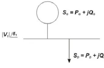
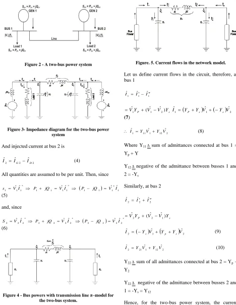
The power flow analysis is a numerical analysis involving the solution of algebraic simultaneous equations, which forms the basis for solution of performance equations [32] [35-36]. A two-bus power system [30] shown in Figure 2, can be used to simplify the development of the power-flow equations. The system consists of two busses connected by a transmission line. One can observe that there are six electrical quantities associated with each bus: PD, PG,

QD, QG,

 

which each bus is shown to have both generation and demand. In reality, not all busses will have power generation. The impedance diagram of the two-bus system is shown in figure 3. In figure 5, the transmission line is represented by a π–model and the synchronous generator is represented by a source behind a synchronous reactance. The loads are assumed to be constant impedance for the sake of representing them on the impedance diagram. Typically, the load is represented by a constant power device, as shown in subsequent figures. Bus power is defined as [30]:

) (

)

( _{1 1 1 1}

1 1

1 SG SD PG PD j QG QD

S      

(1)

And

) (

)

( _{2 2 2 2}

2 2

2 SG SD PG PD j QG QD

S      

(2)

Also, injected current at bus 1 is

1 1 1

ˆ ˆ ˆ

D

G I

I

Figure 2 - A two-bus power system

Figure 3- Impedance diagram for the two-bus power system

And injected current at bus 2 is

2 2 2

ˆ ˆ ˆ

D

G I

I

I   (4)

All quantities are assumed to be per unit. Then, since

 _{1 1} _{1 1}

* 1 1 1 1 * 1 1 1

ˆ ˆ ˆ

ˆ ˆ

ˆ_{I P jQ V I P jQ V I}

V

s        

(5)

and, since

  *

2 2 2 2 * 2 2 2 2 * 2 2 2

ˆ ˆ ˆ

ˆ ˆ

ˆ _{I P jQ V I P jQ V I}

V

S       

(6)

Figure 4 - Bus powers with transmission line π–model for the two-bus system.

Figure. 5. Current flows in the network model.

Let us define current flows in the circuit, therefore, at bus 1

1 1 1

ˆ ˆ

ˆ _{I I}

I   

s

P V V Y

Y

Vˆ₁ ( ˆ₁ ˆ₂)

 Iˆ₁ 









(7)

2 12 1 11 1

ˆ ˆ

ˆ _{Y V Y V}

I  

 (8)

Where Y11 sum of admittances connected at bus 1 =

Yp + Y

Y12 negative of the admittance between busses 1 and

2 = -Ys

Similarly, at bus 2

2 2 2

ˆ ˆ

ˆ _{I I}

I    

s

P V V Y

Y

Vˆ₂ ( ˆ₂  ˆ₁)











2 ˆ ˆ

ˆ _{Y V Y Y V}

I   _s  _p  _s (9)

2 12 1 21 2

ˆ ˆ

ˆ _{Y V Y V}

I   (10)

Y22 sum of all admittances connected at bus 2 = Yp +

Y2

Y22 negative of the admittance between busses 2 and

1 = -Ys = Y12

                   2 1 22 21 12 11 2 1 ˆ V V Y Y Y Y I I (11)

In matrix notation.

Ibus = YbusVbus

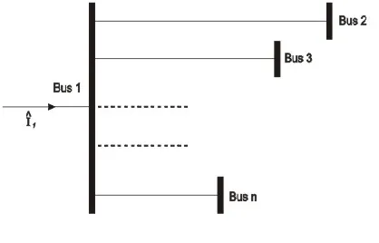
The two-bus system can easily be extended to a larger system. Consider an n-bus system. Figure 2.18a shows the connections from bus 1 of this system to all the other busses. Figure 2.20b shows the transmission line models. Equations (2.73) through (2.86) that were

Figure 6 - An n-bus system

Fig 6, the analysis to an n-bus system derived for the two-bus system can now be extended to represent the n-bus system. This is shown in figure 7.

Figure 7 - The π-model for the n-bus system













12 2 1 1 1 13 1 12 1 ˆ ˆ ... ˆ ˆ ˆ ˆ ˆ ... ˆ ˆ ˆ Ys Ys Ys n p p p V V V V V V Y V Y V Y V I           





(12) n nV Y V Y V Y V Y

Iˆ₁  ₁₁ ˆ₁  ₁₂ ˆ₂  ₁₃ ˆ₃ ... ₁ ˆ

(13)

Where





11 Yp Yp ... Yp Ys Ys ... Ys

Y        

(14)

= sum of all admittances connected to bus 1

ln ln

13 13

12

12 Ys ;Y Ys ;Y Ys

Y      

(15)



ˆ ₍₁₆₎

Also, extending t hepower Eq. (5) to an n-bus system.

j n j jV Y V I V jQ

P ˆ ˆ ˆ

1 1 1 1 1 1 1



Equation (17) can be written for any generic bus i:

n i V Y V jQ P _j n j ij i i

i 1,2,...,

ˆ ˆ 1   



Equation (18) represents the nonlinear power-flow equations. Equation (11) can also be rewritten for an n-bus system:

                                                  n nn n n n n n V V V Y Y Y Y Y Y Y Y Y I I I ˆ ˆ ˆ ˆ ˆ ˆ 2 1 2 1 2 22 21 1 12 11 2 1 (19) Or

Ibus = YbusVbus

             nn n n n n bus Y Y Y Y Y Y Y Y Y Y       2 1 2 22 21 1 12 11

Bus admittance matrix

(20)

The power-flow Eq. (18) can be resolved into the real and reactive parts as follows:

n i V Y V real P n j j ij i

i 1,2, ,

ˆ ˆ 1          



i 1,2, ,

ˆ ˆ Im 1          



Thus, there are 2n equations and 6n variables for the n-bus system. Since there cannot be a solution in such case, 4n variables have to be prespecified. Based on parameter specifications, we can now classify the busses as shown in table 1.

VI. CONCLUSION

This work reveals a comprehensive theoretical framework for implementation and analysis power flow problem. It provides dependable procedures for the mathematical analysis and software implementation of power flow problems. This power flow analysis provides a great deal of insight into the behavior of the power system, in order to ensure economic efficiency and fast return on investment (ROI).

REFERENCES

[1] M. C. Anumaka, “Power flow study on alternating current (ac) power system”. International Journal of Innovative Technology and Research (IJITR). Vol. 2, Issue 4, 2014.

[2] S. H. Low, "Convex relaxation of optimal power flow: A tutorial". 2013 IREP, Symposium on Bulk Power System Dynamics and Control - Ix Optimization, Security and Control of the Emerging Power Grid. pp. 1–06, 2013.

[3] W. Zhang, L. M. Tolbert, "Survey of reactive power planning methods", IEEE Power Engineering Society General Meeting, pp. 1580-1590, 2005

[4] R., Mageshvaran, I.J., Raglend, V., Yuvaraj, P.G., Rizwankhan, T., Vijayakumar, and Sudheera. “Implementation of non-traditional optimization techniques (PSO, CPSO, HDE) for the optimal load flow solution”, TENCON2008-2008 IEEE Region 10 Conference, 19-21 November 2008.

[5] J. R. S. Mantovani, A. V. Garcia, "A heuristic method for reactive power planning", IEEE Trans. Power Syst., vol. 11, no. 1, pp. 68-74, Feb. 1996

[6] Antonio TriasThe embedding load flow method (HELM),EEI Transmission, Distribution, and Metering, Conference Spring 2012, Newport, Rhode Island, April 3, 2012.

[7] M.C., Anumaka,. “Scenario of electricity in Nigeria”. International Journal of Engineering and Innovation Technology (IJEIT) Vol.1, issue 6, pp. 176-183, June.

[8] J.D., Glover, and M.S., Sarma, “Power System Analysis, and Design”. 3rd _{ed. Wandsworth Group. Thomson Learning Inc,} 2012a.

[9] J. Urdaneta, J. F. Gomez, E. Sorrentino, L. Flores, R. Diaz, "A hybrid genetic algorithm for optimal reactive power planning based upon successive linear programming", IEEE Trans. Power Syst., vol. 14, no. 4, pp. 1292-1298, Nov. 1999.

[10] J. Z. Zhu, C. S. Chang, W. Yan, G. Y. Xu, "Reactive power optimization using an analytic hierarchical process and a nonlinear optimization neural network approach", IEE Proc. Generation Transmission and Distribution, vol. 145, no. 1, pp. 89-97, Jan. 1998.

[11] Y. L. Chen, C. C. Liu, "Interactive fuzzy satisfying method for optimal multi-objective Var planning in power systems", IEE Proc. Generation Transmission and Distribution, vol. 141, no. 6, pp. 554-560, Nov. 1994.

[12] C. A. Cazares, "Applications of optimization to voltage collapse analysis", Panel Session: Optimization Techniques in Voltage Collapse Analysis IEEE-PES Summer Meeting, 1998-Jul [13] O.L., Elgerd, “Electric Energy System Theory: An

introduction”, 2nd _{Edition, Mc-Graw-Hill, 2012.}

[14] I.J., Kothari, and D.P., Nagrath, “Modern Power System Analysis”. 3rd _{Edition, New York. 2007.}

[15] J.D., Glover, and M.S., Sarma, “Power System Analysis and Design”, 3rd _{Edition, Brooks/Cole, Pacific Groove. 2002.} [16] B., Slott, and O., Alsac, “Fast Decoupled Load Flow,” IEEE

Trans. On Power Apparatus and Systems. PAS-93, 859-869, 1974.

[17] I.A., Adejumobi, et al., “Numerical Method in Load Flow Analysis: An Application to Nigeria Grid System”,. International Journal of Electrical and Electronics Engineering (IJEEE), 2017.

[18] S., Hadi, “Power System Analysis,” 3rd _{Edition, PSA} Publishing, New York, 2010.

[19] B., Aroop, B., Satyajit, and H., Sanjib, “Power Flow Analysis,” IEEE 57 bus System Using Math-lab. International Journal of Engineering Research and Tech. (IJERT), 3, 2014.

[20] F., Milano, “Continuous newton’s method for power flow analysis” IEEE Trans. On Power Systems 24, 50-57, 2009. [21] J.J., Grainger, and W.D,” Stevenson, Power System

Analysis,”McGraw-Hill, New York, 1994.

[22] W.F., Tinney, and C.E., Hart,” Power Flow Solution By Newton’s Method” IEEE Trans. On power apparatus and system, PAS-86, 1449-1460, 1967.

[23] A. Araposthatis, S. Sastry, P. Varaiya, "Analysis of power flow equation", Int. JournalElec. Power and Energy Syst., vol. 3, no. 4, Oct. 1981.

[24] T. E. DyLiacco, "Real time computer control of power systems", IEEE Proceedings, vol. 62, July 1974.

[25] P. Kundur. Power System Stability and Control. McGraw Hill, New York, 1994

[26] M.C., Anumaka, and C.B., Mbachu, “Modeling Nigerian 330kV Grid for Power System Evacuation and Bus Voltage Improvement”. International Journal of Advances in Science and Technology. Vol.1. No 2, pp. 26- 43, 2013.

[27] B. Stott, "Review of load flow calculation methods", IEEE Proceedings, vol. 62, July 1974.

[28] A. J. Korsak, "On the question of uniqueness of stable load flow solutions", IEEE Trans. Power App. Syst., vol. PAS-91, May/June 1972.

[30] M.C., Anumaka, “|Electric Power System: Analysis of Power Losses and Bus Voltage Improvement in the Nigerian 330KV Interconnected Power System”, Lambert Academic Publishing, Germany, 2015. .

[31] M. Parihar, M.K. Bhaskar, D. Jain, “Long Transmission Line Performance and Model Analysis", National Conference on New Advances in Communications, Networking and Cryptography (NACNC), 28-29 March -2017.

[32] A., Keyhani, A., Abur, and S., Hao, “Evaluation of Power Flow Techniques for Personal Computers. IEEE Transactions on Power Systems, 4, 817-826, 1989.

[33] B., Aroop, B., Satyajlt, and H., Sanjib, Power Flow Analysis on IEEE 57 bus System using Mathlab,” International Journal of Engineering Research Technology (IJERT), 3, 2014.

[34] N., Bhakti, and N., Rajani, Steady State Analysis of IEEE-6 Bus System Using PSAT Power Tool Box. InternationalJournal of Engineering Science and Innovation Technology (IJESIT), 3, 2014.

[35] B., Stott, Review of Load-Flow Calculation Methods. Proceedings of the IEEE, 62, 916-929, 1974.

[36] I.A., Adejumobi, “Numerical Methods in Load Flow Analysis: An Application to Nigeria Grid System” International Journal of Electrical and Electronics Engineering (1JEEE), 3, 2014. [37] S.T. Despotovic, "A new decoupled load flow Method," IEEE

PES summer meeting, Jan 1973, pp 884-891.

[38] S. T. Despotovic, B. S. Babic, and V. P. Mastilovic, "A rapid and reliable method for solving load flow problems," IEEK Trans.Power App. Syst, vol. PAS-90, pp. 123-130, Jan. Feb. 1971.

[39] Brian Stott, "Decoupled Newton Load Flow". IEEE Trans., 1972, PAS-9L pp.1955-19539.

[40] J. E. Van Ness, 'Iteration methods for digital load flow studies," AIEE Trans. (Pown App Syst), vol 78 pp 583-588, Aug. 1959. [41] H. E. Brown, G. K., Carter, H. H. Happ, and C. E Person,

"Z-matrix algorithms in load-flow programs," IEEE Trans Power App, Syst, vol. PAS-87, pp. 807-814, Mar. 1968.

[42] A. F. Giimn and G. W Stagg, "Automatic calculation of load flows," AIEE Trans. (Power App. Syst), vol. 76, pp, 817-828, Oct 1957.

[43] J. B. Ward and. W. Hale, "Digital computer solution of power flow problems," AIEE Trans. (Power App. Syst), vol. 75, pp 398-304, June 1956.

[44] R. J. Brown and "W. F. Tinney, "Digital solutions for large power networks," AIEE Trans (Power App Syst.), vol 76, pp 347-355, June 1957.

[45] Xiao-Ping Zhang, Heng Chen, "Sequence decupled Newton-Raphson three phase load flow", in Proc. IEEETENCON, 1993, pp. 394-397.

[46] VL. Paucar, Marcas J. Rider."Artificial Neural Networks for Solving Power Flow Problems in Electric Power System". Electronic Power. Syst Res. 62, pp.139-144.

[47] A. Arunagiri, B. Venkatesh, K. Kamasamy, “Artificial Neral Network Approach-An Application to Radial Load Flow Algorithm”, IEICE Electronic Express, 206, 3, pp. 353-360. [48] M. Mohatram, P. Tewari, N. Latanath, "Economic load flow

using lagrange neural network", in Proc. Electronics, Communications and Photonics Conference (SIECPC), 2011 Saudi International, pp. 1-7,April 2011,

[49] A. M. Sasson, C. Trevino, and F. Aboytes, ''Improved newton's load flow through a minimization technique," in Proc. IEEE PICA Conf, Boston, 1971.