Wing Design Using SAIL

Scholarly Horizons: University of Minnesota, Morris

Undergraduate Journal

Volume 6 | Issue 2

Article 5

July 2019

Wing Design Using SAIL

Leonid Scott

University of Minnesota Morris

Follow this and additional works at:

https://digitalcommons.morris.umn.edu/horizons

Part of the

Theory and Algorithms Commons

This Article is brought to you for free and open access by the Journals at University of Minnesota Morris Digital Well. It has been accepted for inclusion in Scholarly Horizons: University of Minnesota, Morris Undergraduate Journal by an authorized editor of University of Minnesota Morris Digital Well. For more information, please [email protected].

Recommended Citation

Scott, Leonid (2019) "Wing Design Using SAIL,"Scholarly Horizons: University of Minnesota, Morris Undergraduate Journal: Vol. 6 : Iss. 2 , Article 5.

Cover Page Footnote

This work is licensed under the Creative Commons Attribution- NonCommercial-ShareAlike 4.0

Wing Design Using SAIL

Leonid Scott

Division of Science and Mathematics University of Minnesota, Morris Morris, Minnesota, USA 56267

[email protected]

ABSTRACT

In engineering spaces where modeling is difficult, engineers seek a variety of well performing solutions in order to con-centrate resources on promising areas of the problem space. We call this processillumination. Gaire et al have designed an algorithm specifically for illumination of problem spaces where the underlying model is computationally expensive. This algorithm, Surrogate Assisted Illumination (SAIL) uses anevolutionary algorithmcalled MAP-Elites to do illumina-tion. However, SAIL introduces a Gaussian process to simu-late the computationally expensive model, and Bayesian op-timization for quality control of the Gaussian process. SAIL has demonstrated potential for finding a variety of well per-forming solutions when applied to the design of aerodynamic hulls forvelomobiles. We will walk through each of the com-ponents of the SAIL algorithm, and the results of the velo-mobile experiment.

Keywords

Evolutionary Computation, MAP-Elites, Gausian Processes, Bayesian Optimization

1.

INTRODUCTION

Fluid dynamics stands as one of the most difficult prob-lem spaces to model and thus design in. The equations that govern fluid flow, known as theNavier-Stokes equations, are a set of of partial differential equations with no known so-lution. As a result, aerospace engineers must use extraordi-nary computational power to approximate Navier-Stokes re-sults. High fidelity models of aerodynamic devices can take hours to simulate and still impart noticeable error. Given the difficulty in modeling fluid flow, designing wing shapes is an extraordinary challenge.

Optimization tools aid in this challenge by helping engi-neers at the end of the design cycle by refining a design to what is known as alocal optima. In difficult problem spaces such as fluid dynamics, there is no guarantee that an opti-mizer has found the best possible solution across the entire problem space. However, the optimizer can be very confi-dent that it has found the best solution in one small region. We call the optimal solution across the entire problem space aglobal optima, and an optimal solution in a subsection of

This work is licensed under the Creative Commons Attribution-NonCommercial-ShareAlike 4.0 International License. To view a copy of this license, visit http://creativecommons.org/licenses/by-nc-sa/4.0/.

UMM CSci Senior Seminar Conference, April 2019Morris, MN.

the problem space alocal optima.

In 2014, Autodesk, a producer of modelling and optimiz-ing software found that their software was beoptimiz-ing used in a peculiar way by engineers. Instead of using optimizing tools at the end of the design process to refine designs, engineers used them at the beginning to explore the space of possible designs[2]. Instead of using these tools to find, with great accuracy, one local optima, they were used to find several lo-cal optima throughout the problem space. By finding several local optima, designers could see what tradeoffs are inher-ent in the problem space, and hone in on regions of interest. This process is known asillumination.

Over the course of several years, a research group consist-ing of Adam Gaier, Alexander Asteroth, and Jean-Baptiste Mouret have developed a purpose built algorithm to illumi-nate problem spaces, particularly when models are compu-tationally expensive. This algorithm, known as Surrogate-Assisted Illumination(SAIL) uses a thus far reliable method for exploring problem spaces known as evolutionary compu-tation, albeit in a very specialized form. The goal of SAIL is to produce a series of high performing solutions, across the problem space, to challenging engineering problems.

2.

EVOLUTIONARY ALGORITHMS

SAIL uses a type ofevolutionary algorithm (EA) to ex-plore and exploit the problem space. Evolutionary algo-rithms are stochastic algoalgo-rithms (algoalgo-rithms including ran-domness) inspired by biological evolution. The premise of an evolutionary algorithm is that a population of poten-tial solutions is tested against a model of the problem and assigned a fitness score. The individuals with the best fit-ness scores move onto the next generation and produce “off-spring”. Over many generations the performance against the model will improve until a target performance is obtained, or the algorithm reaches a fixed number of generations.

3.

SAIL ARCHITECTURE

SAIL is made up of three major components: MAP-Elites is the evolutionary algorithm that illuminates problem spaces. Gaussian processes approximate the computationally expen-sive model. Finally, Bayesian optimization enforces quality control of the Gaussian process. This section will explain each of these components in depth before constructing Sur-rogate Assisted Illumination.

3.1

MAP-Elites

MAP-Elites is an evolutionary algorithm developed in April 2015 by Jean-Baptiste Mouret and Jeff Clune [4]. The

pur-1

Scott: Wing Design Using SAIL

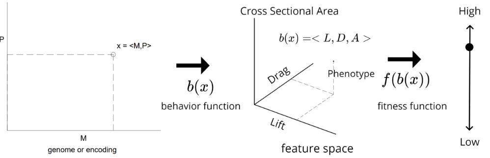
Figure 1: Process of moving from an individual genome to a fitness score.

pose of MAP-Elites is toilluminatethe problem space. That is, to produce a series of high performing solutions that represent different trade offs and insights into the problem space. Before moving into the details of MAP-Elites, it is important to understand the terminology surrounding indi-viduals in MAP-Elites (See Figure 1).

3.1.1

Genotypes

An important aspect in the application of any evolution-ary algorithm is the way that individuals are represented. In engineering contexts, there is a need to represent a physical object in all of its complexities in a compact and understand-able form. In evolutionary algorithms, this representation is referred to as an encoding or a genotype interchangeably. For example, a common way to represent a two dimensional

foil (wing shape) is with a format called the NACA 4 Digit Series [5]. NACA 4 digit foils contain three numbers refering to important geometric features of the foil shape, but also directly relate to foil performance.

Figure 2: Description of NACA 4 Foil.

Figure 2 describes these three values geometrically: M

refers to how “arched” the foil is. P describes where the most “arched” part of the foil exists. Finally,T, refers to the thickness of the foil at its thickest point. Figure 1 shows a

solutions space, the space of all genomes. In this example, we hold thickness constant so the solution space is in two dimensions. With this compact genotype for a 2D foil, it is possible to represent a large range of complex shapes with only three numbers.

3.1.2

Phenotypes

Once we have a representation of an individual, we can start deriving itsbehaviors, orphenotypes. In this example, those behaviors are theliftanddrag of the foil in a certain fluid condition as well ascross-sectional area (the space be-tween the top and bottom lines in Figure 2). In Figure 1, the

feature space, the space of all possible phenotypes, will exist in three dimensions: lift, drag, and cross-sectional area. The function that takes in an individual and returns its pheno-type is known as thebehavior function,b(x).

3.1.3

Fitness

MAP-Elites requires some sort of specific score so that it can definitively tell that one foil is “better” than another. The fitness function f(x), takes an individual and its be-haviors and returns a score quantifying how well it accom-plishes our specified goals. When developing a foil shape, we most certainly care about lift and drag, but for weight and structural reasons, we might also care about the foil’s cross-sectional area. A fitness function that encompasses these behaviors into a single score might look like this:

f(x) =a∗Lift(x)−b∗Drag(x)−c∗Area(x) wherea,b, andcare constants defined by the engineer based on which factors are more important than others. Here,f(x) is set such that a higher fitness score means a foil is better at achieving our goals, but it doesn’t have to be that way. Fitness functions can be setup such that a good score is a: small score, a small absolute value, etc.

3.1.4

MAP-Elites

MAP-Elites works by discretizing the feature space into a set of bins. Each bin in the grid represents tradeoffs between features. For example, the feature space in Figure 3 is split into three sections per dimension, with three dimensions, this results in 27 bins in the feature space. The highlighted box indicates individuals with high lift, medium drag, and medium cross sectional area.

Each generation in MAP-Elites begins by creating an in-dividual from the search space and computing its behaviors using the behavior function. The results of the behavior function will place it in a bin of the feature space. If there is already an individual in that bin, the fitness function will be computed on both individuals, and the individual with the superior fitness will end that generation occupying the bin. If there is no individual in that bin, the new individual simply occupies it.

fea-Figure 3: How MAP-Elites disrectizes a feature space. Here, each of three dimensions is split into three sections, yielding 27 “bins”.

ture space. The individuals who occupy a bin at the end of a generation are known aselites. During each subsequent generation, a new individual is randomly generated. That new individual will compete with the elites from the previ-ous generation for a bin in the feature space.

By default, MAP-Elites creates new individuals by choos-ing a random elite and “tweakchoos-ing” it. This process is called

mutation. Because small changes in the genome of an indi-vidual can result in large changes in behavior, it is common for the mutated individual to compete in a different bin than the parent.

The designer can decide how MAP-Elites terminates. Ter-mination can happen after: A fixed number of generations or computational cost is exceeded. One or many elites have a fitness over a given threshold. Alternatively, after a certain number of bins are filled.

The last point alludes to an important aspect of MAP-Elites: not all bins can always be filled. In our example, physics does not allow a foil to have high lift, zero drag, and minimal cross-sectional area. For this reason, the highest lift, lowest drag, lowest cross-sectional area bin might not be filled. In addition to finding good solutions for a problem, MAP-Elites also offers insights on just where the physics of a problem caps performance of solutions.

3.2

Gaussian Process

Like many evolutionary algorithms, MAP-Elites evaluates the model’s fitness and behavior functions several times per generation. Considering a single MAP-Elites run can involve hundreds of thousands, or even millions of generations, the model needs to be computationally inexpensive. However, in engineering contexts like fluid dynamics, computing lift and drag of a foil in high fidelity can take hours. In these cases, the model is prohibitively computationally expensive for use in traditional evolutionary algorithms.

SAIL avoids computing the model directly most of the time by utilizingsurrogate modelsto approximate the model. Surrogate models strategically execute the model in only limited points of the problem space. They then use this information to extrapolate what other parts of the model should behave like. Gaier et al have chosen to useGaussian processes (GPs) as a surrogate model because they require very few queries from the model in order to start extrap-olating from the problem space. In addition, GP’s include information about how confident they are about the

extrap-olation of a certain point in the problem space.

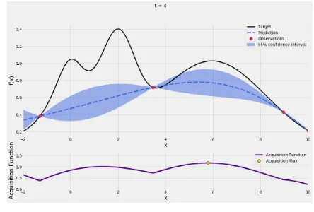
Space constraints limit us from diving into the statistics driving Gaussian processes. Instead, we will walk through how they are used.1 _{Figure 4 shows a Gaussian process that}

is trying to model a target function shown in black. The GP has four observed points to build its model from (shown as red dots in Figure 4). With these observations, the GP can begin to extrapolate what a value of f(x∗) might be for a givenx∗. The GP will return a prediction, and a confidence in its extrapolation off(x∗).

If we extrapolate a large number of points we get Figure 4. The GP prediction for each of these extrapolations form the blue dashed line. We call this dashed line, the mean prediction of the Gaussian process. The confidence at each extrapolation blends into two lines: upper and lower con-fidence intervals. These concon-fidence bounds define the top and bottom of the GP prediction the figure. The confidence bounds in Figure 4 are drawn such that we are 95% certain that the true value of f(x∗) is within these bounds. More-over, for each extrapolated x∗, we are most confident that the true value off(x∗) is on the mean prediction line. From there, the likelihood of the true value off(x∗) drops off with distance from the mean prediction line.

Areas that have low confidence, and a wide spread are said to have high variance. The variance contracts around our observed points, and expands as we get farther away from the observed points. This leads to an important feature of Gaussian processes: Where there is data, we are confident, where there is no data, we are less confident.

3.3

Bayesian Optimization

The fact that Gaussian processes are confident where there is data, and less confident where there is not, allows us to ask an important question: If we were to add another point to our Gaussian process, where would we do it? If our objec-tive is to maximize the function modeled by our Gaussian processes in Figure 4, then our new point can help us do that in one of two ways: First, we could try to pick a point where our prediction is maximized, nearx= 5; this is called

exploiting our problem space. Second, there are two areas between x = 0 tox = 2 and x = 5 to x = 7 with high variance. Selecting a point in this area would improve the overall accuracy of our model, and there might just be a maxima to our function in that region. Selecting a point for this rational is calledexploring the problem space.

1

If you would like to learn the mechanics behind Gaus-sian processes, Dr. Nando de Freitas has a fantastic set of recorded lectures: https://youtu.be/4vGiHC35j9s

3

Scott: Wing Design Using SAIL

Figure 4: A Gaussian processes modelling a function f(x)with four points (top image), and five points on the bottom. One of the observed values is on the far right. For both GP’s, the UCB acquisition function is computed in purple. Taken from [1]

The degree to which we should explore or exploit the prob-lem space is a difficult question. Bayesian optimization at-tempts to balance these objectives by providing a rule for computing the utility of observing another point. There are many different ways of computing utility with Bayesian op-timization; Gair et al decided to use theUpper Confidence Bound Optimizer:

U CB(x) =µ(x) +kσ(x)

The utility of observing a new value from the model, the

U CB(x) at a pointx, is the linear combination of the the mean prediction at a point,µ(x), and some constantk, times the variance,σ(x), at some point. Varyingktunes the model to favor exploration vs exploitation in different quantities. We call the resulting function theacquisition function.

Figure 4 shows how a Bayesian optimization is applied to a Gaussian processes. The UCB, in purple, is computed along the x axis. The top image shows the GP with four observations. At this stage, the model is not doing too well at approximating the true function. Maximizing the acquisi-tion funcacquisi-tion gives us a point with both a high approximated value and a high variance.

We select that point, re-compute the Gaussian processes and rebuild the acquisition function. The updated GP and acquisition function is shown on the bottom image. Again, UCB balances exploration vs exploitation and finds a point with a high predicted value, and high certainty. Using Bayesian optimization allows the GP to model the underlying func-tion with very few points, and make significant progress with each observation.

3.4

SAIL Algorithm

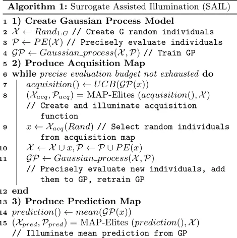
Understanding Gaussian processes and Bayesian optimiza-tion allows us to construct Surrogate Assisted Illuminaoptimiza-tion (SAIL). The pseudocode of SAIL is shown in Algorithm 1. SAIL consists of three phases: 1) Creation of the Gaussian processes, 2) The production of the acquisition map, and 3) The production of the prediction map.

The first stage of the algorithm consists of sampling the problem space and building a Gaussian processes that will model fitness. Recalling the foil terminology used in section 3.1, SAIL would create random individuals withM and P

Algorithm 1:Surrogate Assisted Illumination (SAIL)

1 1) Create Gaussian Process Model

2 X ←Rand1:G// Create G random individuals

3 P ←P E(X)// Precisely evaluate individuals

4 GP ←Gaussian process(X,P)// Train GP

5 2) Produce Acquisition Map

6 whileprecise evaluation budget not exhausted do 7 acquisition()←U CB(GP(x))

8 (Xacq,Pacq) = MAP-Elites (acquisition(),X)

// Create and illuminate acquisition function

9 x← Xacq(Rand)// Select random individuals

from acquisition map

10 X ← X ∪x,P ← P ∪P E(x) 11 GP ←Gaussian process(X,P)

// Precisely evaluate new individuals, add them to GP, retrain GP

12 end

13 3) Produce Prediction Map 14 prediction()←mean(GP(x))

15 (Xpred,Ppred) = MAP-Elites (prediction(),X)

// Illuminate mean prediction from GP

values, compute the precise model for each of them, and use those results to build a Gaussian process.

The second stage of SAIL trains the Gaussian processes by producing anacquisition map. Here, an acquisition func-tion is computed from the Gaussian process using theUpper Confidence Bound (UCB). It is important to note that even though UCB is a linear combination of components, these components are in no way simple shapes. For this reason, the acquisition function will not have an intuitive shape ei-ther. Moreover, the acquisition function reflects the dimen-sionality of the feature space. In a high dimensional feature space, the aquisition function will be a complicated high di-mensional function. Considering this, finding optima in the acquisition function can become a challenge. MAP-Elites is perfectly suited to find not just the global optima of the acquisition function, but illuminate the acquisition function across the entire feature space. The resulting set of high utility individuals is called theacquisition map.

4.

3D FOIL EXPERIMENT: VELOMOBILE

EXPERIMENT

Gaier et al included two experiments in their paper. Due to space constraints, we will only visit the more ambitious of the two: The application of SAIL to design three dimen-sional shapes of aerodynamic hulls forvelomobiles. Velomo-biles, shown in Figure 5, are fully human powered “bicycles”. The cyclists in a velomobile sit in arecumbent position, like one would sit in a paddle boat, and are enclosed in an aero-dynamic hull. The hull allows engineers to carefully craft the airflow around the velomobile to reduce drag. Beause of this reduced drag, velomobiles hold several world speed records for human powered devices.

Figure 5: Milan Velomobile. Taken from [3]

Figure 5 shows how velomobiles have unintuitive hull shapes. The strange contours to these hulls provide an interesting problem space to illuminate. Moreover, the fluid dynamics software that simulates how air moves around the hull shape has high computational cost, stressing the need for a data efficientapproach to illumination. In short, the illumination of velomobile hulls is a good testing ground for SAIL.

Gaier et al encountered several difficulties with this ex-periment. Most prevalently, the data efficient nature of this problem rules out use of MAP-Elites as a control. With MAP-Elite’s heavy reliance on the computationally expen-sive model, illuminating these shapes would take hundreds, if not thousands of hours. Previous experiments in [3] demon-strate SAIL’s ability to create near optimal solutions in fluid dynamic contexts, so the focus shifted from testing SAIL’s ability to compete against other illumination algorithms, to focusing on how different velomobile representations affect performance of the SAIL algorithm. Two representations, or encodings, of velomobile shape, are used in this experiment: a parameterized, and deformed encoding.

4.1

Parameterized Encodings

The parameterized encoding uses a set of aerofoil shapes to create a three dimensional velomobile hull as seen in Fig-ure 6.

Figure 6: Parameterized Encoding. Taken from [3]

There are four foil shapes in the parameterized encoding. The top foil shape, a symmetrical foil, defines the hull at its widest point from above. The mid foil shape represents the foil at it’s centerline. The ridge foil represents the hull where the cyclist’s knees protrude upward. Finally, the rib foil affects how aggressively curved the surface of the hull will be. All in all, this encoding will contain 16 parameters. An advantage of an encoding like this is that each of the 16 parameters directly change the aerodynamic properties of their respective foil shapes.

4.2

Deformation Encodings

Where the parameterized encoding represent key aspects of the shape directly relating to performance, deformed en-codings take another approach. Deformation enen-codings “de-couple the complexity of a the design from the complexity of the representation [3]”. That is, these encodings allow SAIL to find key features of foil performance on its own. Figure 7 shows an example of a deformation encoding:

Figure 7: Deformed Encoding. Taken from [3]

Deformation encodings start with a base design, and sur-round it with a lattice, or grid, of control points. These control points can be shifted in a particular axis. As a con-trol point is moved, the base design will deform to adjust to the shifted control point. Gaier et al allow 16 different points to be altered, each in only one axis.

4.3

Experimental Setup

The goal of this experiment is to see how two features, cur-vature and volume, impact the drag of a velomobile shape. It is known that an increase in volume leads to an increase in drag, but a designer might want to explore how volume impacts drag to accommodate shifting requirements regard-ing volume (the pedalregard-ing mechanism requirregard-ing more space). Moreover, designs with less curvature generally have less drag, but the thin carbon fiber might require additional (heavy) reinforcement to prevent flutter at high speed.

SAIL started with 200 velomobile shapes to train the GP. During each iteration of the illumination phase, 10 individ-uals were chosen from the acquisition map to improve the GP. There were a total of 100 illumination iterations lead-ing to 200 + 10∗100 = 1200 precise evaluations during the illumination phase. The feature map was discretized into a 25 x 25 map, leading to 625 bins.

Fitness was computed as the drag force on the velomobile as it travels at 20 m/s (44.7 mph). A low drag force will represent a better velomobile.

4.4

Results: Design Performance

Figure 8 shows the prediction maps for both the deformed and parameterized encodings as well as a comparison against

5

Scott: Wing Design Using SAIL

the two. In the left two images, a lighter color indicates more drag, and a cooler color indicates less. We are aiming to minimize drag, so darker regions are preferred.

Figure 8: (Left) Prediction maps from deformed and perameterized encodings. (Right) Comparison of the two encodings. Taken from [3]

The deformation encoding has a set of empty bins in the high volume, high curvature section of its prediction map. This is because the deformed encoding is too tightly con-strained to create high volume, high curvature solutions. It’s clear that drag does increase with volume. Encoding con-straints aside, curvature does not seem to impact on drag.

The right side of Figure 8 shows the deformation encod-ings’ successes against the parameterized encoding. Lighter color highlights regions where deformation has a better fit-ness than the parameterized encoding; cooler color indicates the converse. There is only color where there is a significant change in fitness between the two encodings. Deformation does better in the high volume, low curvature region of the feature space, where as the parameterized encoding does better around the edges of the feature space.

4.5

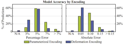
Results: Model Accuracy

After each run, the individuals in the prediction map were precisely evaluated in order to record errors in the final GP model. Figure 9 shows that roughly 60% of the drag calcu-lations for individual’s where within 5% of the computation-ally expensive model. The left side of Figure 9 shows the deformed encoding has slightly lower error than the param-eterized encoding. However, it’s unclear why.

Figure 9: GP error for both encodings. From [3]

4.6

Results: Design Exploration

The two encodings lead to very different looking solutions that occupy the same bins in the prediction map at the end of the SAIL run. Figure 10 shows two sets of similarly performing solutions (one of each encoding) that occupy the same bin. Across the prediction map, the parameterized encoding is taller than its deformation analog.

Gaier et al suspect that parameterized encodings are taller than deformed encodings because they have more freedom to pinch the nose of the velomobile than deformed encodings

Figure 10: Two sets of similarly performing solu-tions that highlights the geometric tendencies of each encoding. The left side includes two similarly performing low volume velombiles. The right in-cludes two similar high volume designs. The red indicates how aerodynamic pressure is distributed over the velomobile shape. Areas of greater inten-sity of red indicate higher aerodynamic pressure. The numbers above the figures refer to drag force of the individual in newtons. Taken from [3]

can. A pinched nose reduces frontal area, thereby reducing pressure on the nose of the velomobile. While deformed designs lack this geometric freedom, they make up for it by smoothing out the shape along the length of the entire velomobile, especially where the ridges meet the hull.

These experiments show how various encodings can reach similarly performing solutions from different directions. More-over, they showcase SAIL’s ability to create a variety of high performing solutions independent of encoding.

5.

CONCLUSIONS

The velomobile experiment demonstrates several of SAIL’s capabilities. They show the potential of SAIL as a powerful algorithm for illuminating problem spaces in computation-ally difficult problem spaces. Moreover, SAIL could be used for testing the limits of various encodings. Before commit-ting to a specific encoding, SAIL can show whether or not that encoding is capable of reaching far areas of the fea-ture space. Moreover, SAIL can give an engineer insights as to how each individual point of variation in the encoding contributes to performance.

A particular advantage of SAIL is that it returns, not only a set of high performing solutions, but also the Gaussian proccess model. This model can be used to gain additional insights into the problem space

Gaier et al mention that a potential bottleneck for SAIL is the behavior function. For example, computing curvature for each velomobile precisely would be too computationally expensive. The authors used a simplified model to compute curvature that was significantly faster. Gaier et al propose the expanded use of surrogate models in the behavior func-tion in cases where the behavior funcfunc-tion is too computa-tionally expensive to run for every individual in a SAIL run.

Acknowledgments

6.

REFERENCES

[1] AdCo Engineering GW. Bayesian optimization. [Online; accessed 8-March-2019].

[2] E. Bradner, F. Iorio, and M. Davis. Parameters tell the design story: Ideation and abstraction in design optimization. InProceedings of the Symposium on Simulation for Architecture & Urban Design, SimAUD ’14, pages 26:1–26:8, San Diego, CA, USA, 2014. Society for Computer Simulation International. [3] A. Gaier, A. Asteroth, and J.-B. Mouret. Data-efficient

design exploration through surrogate-assisted

illumination.Evol. Comput., 26(3):381–410, Sept. 2018. [4] J.-B. Mouret and J. Clune. Illuminating search spaces

by mapping elites.

[5] Wikipedia. NACA airfoil — Wikipedia, The Free Encyclopedia, 2019. [Online; accessed 17-April-2019].

7

Scott: Wing Design Using SAIL