The Mathematica® Journal
Symbolic-Numeric
Algebra for Polynomials
Kosaku Nagasaka
Symbolic-Numeric Algebra for Polynomials (SNAP) is a prototype package that includes basic functions for computing approximate algebraic proper-ties, such as the approximate GCD of polynomials. Our aim is to show how the unified tolerance mechanism we introduce in the package works. Using this mechanism, we can carry out approximate calculations under certified tolerances. In this article, we demonstrate the functionality of the currently released package (Version 0.2), which is downloadable from wwwmain.h.kobe-u.ac.jp/~nagasaka/research/snap/index.phtml.en.
‡
Introduction
Recently, there have been many results in the area of symbolic-numeric algo-rithms, especially for polynomials (for example, approximate GCD for univariate polynomials [1, 2, 3, 4] and approximate factorization for bivariate polynomials [5, 6, 7, 8]). We think those results have practical value, which should be com-bined and implemented into one integrated computer algebra system such as
Mathematica. In fact, Maple has such a special package called SNAP (Symbolic-Numeric Algorithms for Polynomials). Currently, ours is the only such package available for Mathematica.
We have been developing our SNAP package for Mathematica, which is an abbreviation for Symbolic-Numeric Algebra for Polynomials. We use algebra to mean continuous capabilities of approximate operations; for example, computing an approximate GCD between an empirical polynomial and the nearest singular polynomial computed by SNAP functions of another empirical polynomial. This continuous applicability is more important for practical computations than the number of algorithms that are already implemented, especially for average users.
Our aim is to provide practical implementations of SNAP functions with a unified tolerance mechanism for polynomials like Mathematica’s floating-point numbers or Kako and Sasaki’s effective floating-point numbers [9]. Our idea is very simple. We only have to add new data structures representing such polynomi-als with tolerances and basic calculation routines and SNAP functions for the structures. At this time, only simple tolerance representations (l2-norm, l1-norm,
Features that are new in Version 0.2 [10, 11], include:
Ë SNAP structures for multivariate polynomials that have more than one variable.
Ë Basic functions that can operate with multivariate polynomials.
Ë New compatibilities with the built-in functions PolynomialReduce and D.
Ë New SNAP functions, such as CoprimeQ, AbsolutelyIrreducibleQ, SeparationBound, Factor, and FactorList.
·
Difference Between Numerical and Algebraic Computations
Let us consider a typical numerical computation—finding numerical roots:
In[1]:= System‘NSolvex^ 210, x, 20
Out[1]= x 1.0000000000000000000,x1.0000000000000000000
We might assume that polynomials that are close have roots that are close.
In[2]:= System‘NSolvex^ 21.0000000000001‘200, x, 20
Out[2]= x 1.0000000000000500000,x1.0000000000000500000
If this argument is not correct, the problem is called “numerically unstable.” Hence, “numerical stability” of the given problem and “significant digits” of the calculated solutions are important in numerical computations. Mathematica’s accuracy and precision tracking system are very useful for this purpose and are based on the concept that the higher precision used, the closer the solutions.
Unfortunately, this concept may not be correct for algebraic computations. Let us consider a factorization:
In[3]:= System‘Factorxyxy0.0000000001‘‘16
Out[3]= 1.000001.0000010101.00000 x21.00000 y2
We cannot factor this polynomial if we increase the precision of the computation because algebraic properties are generally not continuous. Forward and back-ward error analyses may not be the solution, though they can be of supplemental use. The previous polynomial, for example, can be either reducible or irreduc-ible, and we may not be able to know which property is correct.
We note that there are two approaches to operating with empirical polynomials in an extreme instance—using inexact or exact approximations. For example, let us consider factoring bivariate polynomials. The following numerical polynomial is reducible if we rationalize its coefficients up to machine precision:
(1)
fHx, yL= -7.+7.x2 -1.x3+1.x5+15.y+7.x y-1.x2 y+
In[4]:= System‘Factor77 x2x3x515 y7 x y
x2y2 x3yx4y2 y22 x y2x3y22 x y3x2y3
Out[4]= 1x22 yx y 7x3yx y2
This factorization is fine. The problem is operating with the following polyno-mial (we added small perturbation terms to the previous polynopolyno-mial):
(2)
f Hx, yL=
-7.+7.x2-1.x3+1.x5+15.y+7.x y-1.x2 y+2.x3 y+1.x4 y
-2.y2-2.x y2+1.x3 y2+2.x y3+1.x2 y3+0.0000001x-0.0000001
In general, we may not know whether these perturbation terms are numerical errors or actually exist in the polynomial. The inexact approximation approach tries to factor numerically, regardless of significant digits or magnitude of errors. Although we can check its backward error after calculations, we cannot know if the backward error is globally minimized or if the number of factors is globally maximized. Moreover, there is a possibility that an algorithm cannot find appro-priate factors even if there are approximate factors.
Therefore, to do algebraic operations, we have to guarantee the properties for all possible polynomials that are sufficiently close to the given polynomial. For example, assuming the precision is 16, the polynomial set of the polynomial (2) includes the following polynomials:
(3)
f Hx, yL= -7.00000000000000001+7.x2-1.x3+1.x5+
15.y+7.x y-1.x2 y+2.x3 y+1.x4 y-2.y2-2.x y2+
1.x3 y2 +2.x y3+1.x2 y3+0.0000001x-0.0000001
(4)
f Hx, yL= -6.99999999999999999+7.x2-1.x3+1.x5+
15.y+7.x y-1.x2 y+2.x3 y+1.x4 y-2.y2-2.x y2+
1.x3 y2 +2.x y3+1.x2 y3+0.0000001x-0.0000001
Using exact approximations tries to guarantee such properties. However, this approach is more difficult than the first, because we have to guarantee an alge-braic property of an infinite number of polynomials that are sufficiently close to the given polynomial.
‡
Tolerance Mechanisms and Implementations
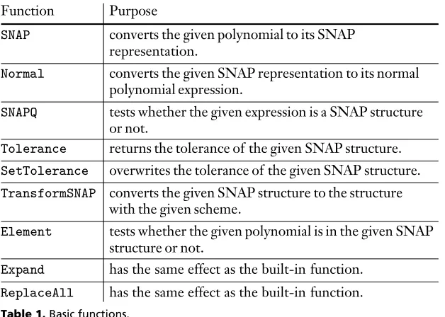
Function Purpose
SNAP converts the given polynomial to its SNAP representation.
Normal converts the given SNAP representation to its normal polynomial expression.
SNAPQ tests whether the given expression is a SNAP structure or not.
Tolerance returns the tolerance of the given SNAP structure. SetTolerance overwrites the tolerance of the given SNAP structure. TransformSNAP converts the given SNAP structure to the structure
with the given scheme.
Element tests whether the given polynomial is in the given SNAP structure or not.
Expand has the same effect as the built-in function.
ReplaceAll has the same effect as the built-in function.
Table 1. Basic functions.
·
Tolerance Mechanisms
We introduce the following data structures for empirical polynomials. They are very simple, but there is no system in which we can automatically use these structures in a way similar to Mathematica’s floating-point numbers or Kako and Sasaki’s effective floating-point numbers [9]. These structures are different from those used in the previous version of this package [10, 11]. The latest version can operate on polynomials that have more than two variables (bivariate or multivari-ate polynomials).
Definition 1 (SNAP Structures). We define the following SNAP structures (like sets of neighbors) for approximate polynomials for the given polynomial
fHu1, … , urL œ @u1, … , urD and tolerance e œ :
(5)
PpHf, eL=9êêêf »êêêf œ@u1, … , urD,
degu fêêê=degu f H"uœ8u1, … , ur<L, °f -êêêf¥p § e=,
where °f¥p denotes coefficient vector norms for polynomials:
(6) °f¥p =HSi†fi§pL
1
ÅÅÅÅÅp, f = S i fiu1
ei1 u
r eir.
In the rest of this article, P*Hf,eL means any P2Hf,eL, P1Hf,eL, or P¶Hf,eL.
Remark 1. You might think that the following definition is better than the previous definition:
(7)
P*Hf, eL=8fêêê»êêêf œ@u1, … , urD,
However, this definition produces strange results. For example, let e be an arbitrary small positive real number and f be the following polynomial:
(8)
f = fnxn +fn-1xn-1++f1x+f0, fi œ, †fn§§ e.
For this polynomial, P*Hf,eL includes polynomials that have n roots (counting multiplicities) and also polynomials that have at most n-1 roots. Moreover, one might want to preserve more than total degree in the multivariate case (sometimes which is called triangle degree while it is called rectangle degree in the definition 1). Those degree models are too advanced for the current results in this research area and they cause unusual results for the known algorithms; hence, we use the expressions of Definition 1.
The coefficient vector norms for polynomials have properties similar to normal vector norms (see [12] for a discussion of these basic properties); hence, we have the following corollary.
Corollary 1. We have the following properties:
(9)
P2Hf, eLŒP1If, e è!!!!!!!!!!!!!!!!!!!!!!!!!Pi=1r Hei+1L M,
(10)
P2Hf, eLŒP¶Hf, eL,
(11)
P1Hf, eLŒP2Hf, eL,
(12)
P1Hf, eLŒP¶Hf, eL,
(13)
P¶Hf, eLŒP2If, e è!!!!!!!!!!!!!!!!!!!!!!!!!Pi=1r Hei+1L M,
(14)
P¶Hf, eLŒP1Hf, e Pi=1r Hei+1LL,
where ei denotes the degree of fHu1, … , urL with respect to ui.
Lemma 1. We have the following properties for polynomials fHu1, … , urL and hHu1, … , urL:
(15)
" êêêf œP2Hf,efL, "h
êê
œP2Hh,ehL, f
êêê µêêhœ
P2If µh,è!!!!!!!!!!!!!!!!!!!!!!!!!!!!!!!!min8Pri=1Hei+1!!!!!!!!!!!!!!!!!!!!!!!!!!!!!!!!L,Pi=1r Hdi+1L<H°f¥2 eh+°h¥2 ef + ef ehLM,
(16)
" êêêf œP1Hf,efL, "h
êê
œP1Hh,ehL, f
êêê
µêêhœP1Hf µh,°f¥1 eh+°h¥1 ef + ef ehL,
(17)
"êêêf œP¶Hf,efL, "h
êê
œP¶Hh,ehL, f
êêê µêêhœ
P¶Hf µh, min8Pi=1r Hei+1L,Pi=1r Hdi+1L<H°f¥1 eh+°h¥1 ef + ef ehLL,
Proof of Lemma 1. The lemma is proved by the following properties of vector and matrix norms [12], since any multiplication of polynomials can be done as matrix multiplications:
(18) °A¥2 §°A¥F,
(19) °A¥1 =max1§j§nSi=1m †aij§,
(20) °A¥¶=max1§i§mSnj=1†aij§,
where °A¥p denotes matrix p-norms for matrix A of size mµn. ·
Lemma 2. If the following relation holds for polynomials fHu1, … , urL and hHu1, … , urL,
(21)
"êêêf œPpHf,efL, "h
êê
œPpHh,ehL,
deguHêêêf +êêhL=max8degu f, deguh< H"uœ8u1, … , ur<L,
we have the following properties:
(22)
" êêêf œPpHf,efL, "h
êê
œPpHh,ehL, f
êêê
+êêhœPpHf +h,ef + ehLª9g»gœ@u1, … , urD, degug=
max8degu êêêf, deguêêh< H"uœ8u1, … , ur<L, °Hf +hL-g¥p § ef + eh=,
where ei and di denote the degree of fHu1, … , urL and hHu1, … , urL with respect to ui, respectively, and p=1, 2,¶.
Proof of Lemma 2. The lemma is directly proved by the triangle inequality for norms. ·
The condition of Lemma 2 is necessary for ensuring equalities for degrees in
P*Hf +h,ef + ehL. Without the condition, unusual results as in Remark 1 may
occur. However, for example, we have to operate with the following computation and determine the set S. This is important especially for divisions (quotient and remainder) and reductions (for non-univariate polynomials):
(23)
"gœP*Hf,eL,"hœP*Hf,eL, g-hœS.
We introduce a simple rule to handle this. If the norm of the leading coefficients of the representative polynomial f, with respect to ui, is not larger than the tolerance e, then we rewrite the SNAP structure as follows:
(24)
P*Hf,eL fl P*Hfnew,eL=8g»gœ@u1, … , urD, degug=degu fnewH"uœ8u1, … , ur<L, °fnew -g¥2 § e<,
where fnew denotes f - (all the leading monomials of f, with respect to ui).
·
Tolerance Implementations
According to the previous definitions, we have implemented the structures, basic operations (addition and multiplication) on the structures, and functions that transform one structure into another.
We define the following expression to represent the SNAP structures P2Hf,eL,
We define the following expression to represent the SNAP structures P2Hf,eL,
P1Hf,eL, and P¶Hf,eL, where scheme can be AbsolutePolynomial2Norm, AbsolutePolynomial1Norm, and AbsolutePolynomialiNorm, respectively. In a future release, other schemes will be implemented.
SNAPf,,u1,e1, ,ur,er,scheme
Using this structure, we have implemented basic functions provided by the mechanisms and now show some of their expressions. We note that the package also provides functions that automatically transform the given polynomial to the previous representation.
TransformSNAPSNAPf_, epsf_,x_Symbol, n_, yz___, AbsolutePolynomial2Norm, AbsolutePolynomialiNorm:
SNAPf, epsf,x, n, yz, AbsolutePolynomialiNorm
NormalSNAPf_, epsf_,x_Symbol, n_, yz___, scheme_:f
SNAP:SNAPf_, epsf_,x_Symbol, n_, yz___, scheme_:
SNAPf, epsf,x, n, yz, scheme
SNAPg_, epsg_, varsg_List, scheme_
SNAPh_, epsh_, varsh_List, scheme_^:
SNAPgh, epsgepsh, maxvarslistvarsg, varsh, scheme SNAPg_, epsg_, varsg_, scheme_f_? NotSNAPQ ^:
SNAPg, epsg, varsg, schemeSNAPf
ToleranceSNAPf_, epsf_, vars_, scheme_:epsf
One aim of the package is providing an environment in which we use SNAP structures transparently, like Mathematica’s floating-point numbers; hence, we have implemented the following Format code.
FormatSNAPf_, e_, variables_, scheme_:Nf
In this version, we suppose that the basic four operations between Mathematica’s bigfloat numbers and its interval arithmetic guarantee the precision of their results, since basically we use Mathematica’s own arithmetic for estimations. All the implementations depend on Mathematica’s accuracy and precision tracking system, though in our implementation, we round up all the error parts in case our assumption is incorrect.
·
Tolerance Examples
Next we show some examples of the SNAP tolerance mechanism. This loads the package.
In[5]:= Needs"SNAP‘"
This package includes routines which provide SNAP functionalities. The version of this package
This gives a SNAP structure. The output looks like a normal expression.
In[6]:= gSNAPx^55.503 x^ 49.765 x^37.647 x^22.762 x0.37725
Out[6]= 0.377252.762 x7.647 x29.765 x35.503 x4x5
This gives the FullForm of the previous SNAP structure.
In[7]:= FullFormg
Out[7]//FullForm=
SNAPPlusRational1509, 4000, TimesRational1381, 500, x, TimesRational7647, 1000, Powerx, 2,
TimesRational1953, 200, Powerx, 3,
TimesRational5503, 1000, Powerx, 4, Powerx, 5, 1.537912594467730969706440230810229‘14.303315010757448*^-15, ListListx, 5, AbsolutePolynomial2Norm
The error bound of this SNAP structure, which is a a set of polynomials, is given by Tolerance.
In[8]:= Toleranceg
Out[8]= 1.537912594467731015
Each calculation enlarges its error bound.
In[9]:= g2gg
Out[9]= 0.377252.762 x7.647 x29.765 x35.503 x4x52
In[10]:= Toleranceg2
Out[10]= 1.046375127452241013
By using Element, we can check whether a polynomial is included in the given SNAP structure or not. The error bound of the following SNAP structure is about 1.53791µ10-15; hence, we have these results.
In[11]:= ElementNormalg1.5*^-15, g
Out[11]= True
In[12]:= ElementNormalg1.6*^-15, g
Out[12]= False
Normal gives corresponding representative polynomials in the normal form.
In[13]:= Normalg FullForm
Out[13]//FullForm=
PlusRational1509, 4000, TimesRational1381, 500, x, TimesRational7647, 1000, Powerx, 2,
TimesRational1953, 200, Powerx, 3,
TimesRational5503, 1000, Powerx, 4, Powerx, 5
In[14]:= Expandg2
Out[14]= 0.1423182.08393 x13.3983 x249.6097 x3116.57 x4 180.499 x5185.042 x6122.768 x749.813 x811.006 x9x10
Any result of a substitution for a SNAP structure also has a guaranteed accuracy.
In[15]:= g3g2. x1
Out[15]= 731.93244306250
In[16]:= Toleranceg3
Out[16]= 1.151012640197511012
We show the situation discussed in the last paragraph of the Tolerance Mecha-nisms subsection.
In[17]:= g
Out[17]= 0.377252.762 x7.647 x29.765 x35.503 x4x5
In[18]:= gx^5
SNAP::invalid: Tolerance is larger than the
representative leading coefficient: 0.‘1.537912594467731‘*^-15.
Out[18]= 0.377252.762 x7.647 x29.765 x35.503 x4
Because this rewriting can be important for users, this package generates the displayed warning.
‡
Other Basic Operations
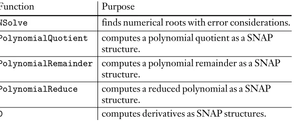
We implemented other basic operations: a polynomial division (quotient and remainder), reductions (for non-univariate polynomials), and root-finding with error considerations.
Function Purpose
NSolve finds numerical roots with error considerations. PolynomialQuotient computes a polynomial quotient as a SNAP
structure.
PolynomialRemainder computes a polynomial remainder as a SNAP structure.
PolynomialReduce computes a reduced polynomial as a SNAP structure.
D computes derivatives as SNAP structures.
·
Polynomial Division (Univariate Case)
Let fHxL and gHxL be the following polynomials of degrees n and m, m§n, with tolerances ef and eg, respectively:
(25)
f HxL= fnxn+ fn-1xn-1++ f1x+f0, fi œ, gHxL=gmxm+gm-1xm-1++g1x+g0, gi œ.
Dividing fHxL by gHxL is defined as follows, with polynomials qHxL and rHxL:
(26)
f HxL=qHxLgHxL+rHxL, degq=n-m, degr<m.
For SNAP structures, we have to check that the polynomials êêqHxL and êêrHxL for the given fêêêHxL and êêgHxL are properly related to qHxL and rHxL:
(27)
f
êêê
HxL=êê qHxLêê gHxL+êê rHxL, degqêê =n-m, degrêê <m, êêêf œP*Hf,efL, êê œg P*Hg,egL.
We have the following corollaries [11]. Note the discussion at the end of the Tolerance Mechanisms subsection.
In these corollaries, G is the Hn+1LµHn+1L matrix:
(28)
G=
i
k jjjjj jjjjj jjjjj jjjjj jjjjj jj
gm 0 0 0
gm-1 gm ª ª
ª gm-1 ª ª
g0 ª 0 ª
ª ª gm 0
0 gm-1 gm
y
{ zzzzz zzzzz zzzzz zzzzz zzzzz zz
.
Corollary 2. If the following expression holds,
(29)
s2è!!!!!!!!!!!n+1 eg<1, s2 =°G-1¥2,
we have
(30)
"êêêf œP2Hf,efL, "êê œg P2Hg,egL, êê œq P2Hq,eqL, êê œr P2Hr,erL
eq= s2Ief +è!!!!!!!!!!!n+1 egH°q¥2+ s2 efL ë I1- s2è!!!!!!!!!!!n+1 egMM,
er = ef +$%%%%%%%%%%%%%%%%%b n
ÅÅÅÅÅÅ
2r+1H°g¥2 eq+°q¥2 eg+ eg eqL.
Corollary 3. If the following expression holds,
(31)
we have
(32)
" êêêf œP1Hf,efL, "êê œg P1Hg,egL, qêê œP1Hq,eqL, rêê œP1Hr,erL, q
êêêêêê œP1Hq,eqL, êê œr P1Hr,erL,
eq= s1Hef + egH°q¥1+ s1 efL ê H1- s1egLL,
er = ef +°g¥1 eq+°q¥1 eg+ eg eq.
Corollary 4. If the following expression holds,
(33)
s¶Hn+1L eg<1, s¶=°G-1¥¶,
we have
(34)
"êêêf œP¶Hf,efL, "êê œg P¶Hg,egL, êê œq P¶Hq,eqL, êê œr P¶Hr,erL,
eq= s¶Hef +Hn+1L egH°q¥¶+ s¶ efL ê H1- s¶Hn+1L egLL,
er = ef +Jb n
ÅÅÅÅÅÅ
2r+1NH°g¥¶ eq+°q¥¶ eg+ eg eqL.
·
Polynomial Reduction (More than One Variable Case)
Since the SNAP structure is extended to multivariate polynomials in this version, we introduce polynomial reductions. Because a reduction can be done by two multiplications and one subtraction, we just reduce polynomials by ordinary algorithms using the SNAP structures introduced in the previous section. Note that we assume that the given polynomial basis is a Gröbner basis for any possi-ble combinations of polynomials in the basis, and the result, including tolerance, is dependent on a specified term order.
·
Root Finding with Error Considerations
There are many root-finding methods. Basically, Mathematica uses the Jenkins– Traub method. Since those roots found by numerical methods may not be the exact ones, we have to consider numerical errors after calculations. For example, Smith [13] studied error bounds for numerical roots.
However, working with polynomials with errors in their coefficients extends the problem. Terui and Sasaki [14] studied an extended version of Smith’s work, by which we can bound errors included in numerical roots of polynomials with errors on their coefficients and for polynomials represented as SNAP structures.
Lemma 3 (Statement in [14]). For any polynomial fêêêHxLœP*Hf,eL, we have
(35)
†zi- z
êê
p HiL§§n
†f HziL§+ e⁄nj=0†zi§j
ÅÅÅÅÅÅÅÅÅÅÅÅÅÅÅÅÅÅÅÅÅÅÅÅÅÅÅÅÅÅÅÅÅÅÅÅÅÅÅÅÅÅÅÅÅÅÅÅÅÅÅÅÅÅÅÅÅÅÅÅÅÅÅÅÅÅÅÅÅÅÅÅÅÅÅÅÅÅÅÅÅ
H†fn§+ eL°¤nj=1,≠iHzi- zjL•
,
where n denotes the degree of fHxL, z1, … , zn and z
êê
pH1L, … , z
êê
pHnL are the roots of fHxL and fêêêHxL, respectively, pHiL is a permutation of 81, … , n< that minimizes the maximum distance between the roots: maxi†zi- z
êê
·
Partial Derivation with Error Considerations
Computing the partial derivatives of the given polynomial is also important. We have the following trivial lemma to calculate the derivatives of SNAP structures.
Lemma 4. For any polynomial fêêêHu1, … , urLœP*Hf,eL, we have
(36)
∂êêêf Hu1, … , urL
ÅÅÅÅÅÅÅÅÅÅÅÅÅÅÅÅÅÅÅÅÅÅÅÅÅÅÅÅÅÅÅÅÅÅÅÅÅÅÅÅÅÅÅÅÅÅÅÅÅÅÅÅ
∂ui œP*ikjjj
∂f Hu1, … , urL
ÅÅÅÅÅÅÅÅÅÅÅÅÅÅÅÅÅÅÅÅÅÅÅÅÅÅÅÅÅÅÅÅÅÅÅÅÅÅÅÅÅÅÅÅÅÅÅÅÅÅÅ
∂ui , e µdegui f y {
zzz Hi=1, … , rL.
·
Examples
Here we show some examples of basic operations of the package using the previous polynomial.
In[19]:= g
Out[19]= 0.377252.762 x7.647 x29.765 x35.503 x4x5
The following examples give all the roots of the given representative polynomial with or without considerations of the error bound. We recommend comparing the following two results of NSolve and System‘NSolve. NSolve with a SNAP structure considers all the possible polynomials within the structure; hence, their tolerances are larger than that of NSolve without a SNAP structure.
This gives a result with error considerations according to Lemma 3.
In[20]:= NSolveg0, x
Out[20]= x 3.00007208113,x 0.9989903849,x 0.54121518, x 0.481361180.02946454,x 0.481361180.02946454
In[21]:= Tolerancex. %
Out[21]= 1.173590672098831012, 3.58892600505511011,
6.8881497758683109, 6.9645254663057109, 6.9645254663057109
This gives a result without error considerations.
In[22]:= System‘NSolveNormalg0, x
Out[22]= x 3.00007,x 0.99899,x 0.541215,
x 0.4813610.0294645,x 0.4813610.0294645
In[23]:= Tolerancex. %
Out[23]= 3.33074910000821016, 1.109102126694171016,
6.00869556830521017, 5.35418495811501017, 5.35418495811501017
To show division examples, define the following two polynomials.
In[24]:= g2Expandgg
Out[24]= 0.1423182.08393 x13.3983 x249.6097 x3116.57 x4 180.499 x5185.042 x6122.768 x749.813 x811.006 x9x10
In[25]:= hx^3Random
Out[25]= 0.465024x3
This gives the quotient and remainder of g2 by h with error considerations. Note that though h is not in the SNAP structure, it is automatically transformed into it and SNAP functions are overloaded because the built-in functions are not compatible with such arguments including a SNAP structure.
This gives the quotient and remainder of g2 by h with error considerations. Note that though h is not in the SNAP structure, it is automatically transformed into it and SNAP functions are overloaded because the built-in functions are not compatible with such arguments including a SNAP structure.
In[26]:= PolynomialQuotientg2, h, x, PolynomialRemainderg2, h, x
Out[26]= 34.059359.6968 x157.335 x2179.924 x3122.303 x4 49.813 x511.006 x6x7, 15.980725.6765 x59.7661 x2
These commands are the same for univariate polynomials.
In[27]:= PolynomialReduceg2,h,x
Out[27]= 34.059359.6968 x157.335 x2179.924 x3122.303 x4 49.813 x511.006 x6x7, 15.980725.6765 x59.7661 x2
In the next example, PolynomialRemainder gives a pseudo-zero number since g can divide g2. However, these polynomials have their error bounds, and we cannot argue that its remainder is completely zero; hence, the following warning messages are generated.
In[28]:= g3, g4PolynomialQuotientg2, g, x, PolynomialRemainderg2, g, x
SNAP::invalid: Tolerance is larger than the
representative leading coefficient: 0.‘1.0292162141035616‘*^-6.
General::stop: Further output of
SNAP::invalid will be suppressed during this calculation.More. . .
Out[28]= 0.377252.762 x7.647 x29.765 x35.503 x4x5, 0.106
SNAP functions give normal Mathematica numbers if their degrees are not larger than zero.
In[29]:= SNAPQg3, SNAPQg4
Out[29]= True, False
Each operation or calculation enlarges error bounds; hence, tolerances of the roots also get larger.
In[30]:= NSolveg30, x
Out[30]= x 3.00007,x 0.99899,x 0.5412, x 0.48140.0295,x 0.48140.0295
In[31]:= Tolerancex. %
Out[31]= 1.76394520485190106, 3.67660059293547106,
0.0000641619768854552, 0.0000561916017665273, 0.0000561916017665273
In[32]:= NSolveg20, x
SNAP::multipleroots: The given representative polynomial
has multiple roots. Tolerances of the roots can not be computed.
Out[32]= x 3.000072,x 3.000072,x 0.99899,
x 0.99899,x 0.54,x 0.54,x 0.480.03, x 0.480.03,x 0.480.03,x 0.480.03
In[33]:= Tolerancex. %
Out[33]= 4.77743842704102107, 4.77743842704538107, 1.63209073103228106, 1.63209073944919106,
0.00376341857130941, 0.00376343263094951, 0.00233327894319648, 0.00233327894319648, 0.00233326644754287, 0.00233326644754287
Partial derivatives also can be computed in SNAP structures.
In[34]:= g2dDg2, x
Out[34]= 2.0839326.7966 x148.829 x2466.282 x3902.495 x4 1110.25 x5859.373 x6398.504 x799.054 x810. x9
In[35]:= NSolveg2d0, x
Out[35]= x 3.00007208,x 2.5308273,x 0.9990,
x 0.8692,x 0.101,x0.101,x0.101, x 0.1010.101,x 0.1010.101
In[36]:= Tolerancex. %
Out[36]= 8.1322107325183109, 2.16884179842690108, 0.0000106535444881950, 0.0000474506566469721, 0.4545922961971249, 12.83683482913959, 10.16786064649990, 0.3798417168646968, 0.3798417168646968
The tolerance correcting method used in SNAP computes subtractions among close numbers so it requires a certain precision. In this case, working precision is not enough; hence, we increase it.
In[37]:= NSolveg2d0, x, 32
Out[37]= x 3.000072081,x 2.530827278,x 0.998990385, x 0.86922548,x 0.541215,x 0.50942,x 0.49292, x 0.4813610.029465,x 0.4813610.029465
In[38]:= Tolerancex. %
Out[38]= 1.426709389682831010,
‡
Symbolic-Numeric Algorithm Implementation
Using the basic features, we have started to modify and implement known symbolic-numeric algorithms. In the current implementation, only one algo-rithm for each computation is used. Other algoalgo-rithms will be implemented in the near future.
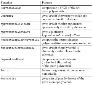
Function Purpose
PolynomialGCD computes ane-GCD of the two given polynomials.
CoprimeQ givesTrueif the two polynomials are coprime within the tolerance. ApproximateDivisorQ givesTrueif the first argument is
approximately divisible by the second. ApproximateQuotient gives a quotient if
ApproximateDivisorQisTrue. NearestSingularPolynomial computes the nearest singular
polynomialHtolerance is not consideredL. AbsolutelyIrreducibleQ givesTrueif the polynomial is
absolutely irreducible within the tolerance.
SeparationBound computes a separation bound
Hor irreducibility radiusL of the given polynomial.
Factor factors the given monic polynomial numerically.
FactorList gives a list of pseudo-factors of the given monic polynomial.
Table 3. Symbolic numeric functions.
·
Approximate GCD and Divisors (Univariate Case)
From the early historical period of symbolic-numeric computations, various approximate GCDs have been studied. The problem treated here is very simple: for the given polynomials gHxL and hHxL and the tolerance e, find a polynomial
fHxL of maximal degree that satisfies
(37)
$êê gHxLœP*Hg, e°g¥*L, $hêêHxLœP*Hh, e°h¥*L, f HxL »êê gHxL, f HxL »hêêHxL,
We note that there are also other approximate GCDs that have slightly different definitions and approximate GCDs of multivariate polynomials. Those approxi-mate GCDs will be implemented in a future release.
Considering approximate GCDs, the following concept of an e-divisor is useful. For the given polynomial gHxL and the tolerance e, we call a polynomial fHxL an
e-divisor of gHxL if fHxL satisfies
(38)
$êê gHxLœP*Hg, e°g¥*L, f HxL »êê gHxL,
where * denotes 2, 1, or ¶. Moreover, in this package, we call the quotient of
g
êêHxL by fHxL an e-quotient of gHxL by fHxL. These concepts are used in Pan’s
algorithm, and currently we have only implemented the 2-norm case.
Note that, theoretically, e-GCD, e-divisor, and e-quotient are exact polynomials, since only the given polynomials have perturbation parts, and e-GCD, e-divisor, and e-quotient are treated as exact polynomials in those computations. However, due to numerical errors, in this package, e-GCD, e-divisor, and e-quotient are treated as SNAP structures.
We also provide a coprimeness check function that uses the well-known fact that if the Sylvester matrix of the given two polynomials has full rank, then they are coprime [15].
·
Nearest Singular Polynomial (Univariate Case)
The nearest singular polynomial [16, 17, 18] of fHxL is the nearest polynomial
f
êêê
HxL that has a double root, minimizes °fHxL-êêêfHxL¥, and has the same degree as
fHxL. A similar problem that finds the nearest polynomial with constrained roots has been studied in [19, 20].
In this package, finding the nearest singular polynomial can be written as follows.
For the given polynomial fHxL and tolerance e, find a polynomial êêêfHxL satisfying
(39)
f
êêê
HxLœP*Hf, eL, $cœ, Hx-cL2» fêêêHxL,
where * denotes 1, 2, or ¶; if the output is False, the nearest singular polyno-mial does not exist in the given SNAP structure. The current version of the package solves this problem using the known algorithm [18], so the command can only solve the problem for the 2-norm case. The constrained roots version of the problem will be solvable in a future release.
Note that the current implementation outputs a normal polynomial (not in a SNAP structure) and the given tolerance for the command corresponding to the nearest singular polynomial does not have the same meaning as the other com-mands of the SNAP package. For more information, see [18].
·
Irreducibility Testing for Bivariate Polynomials
Conventional ordinary factorization algorithms may always output “absolutely irreducible” for numerical or empirical polynomials, since the given polynomial may have error parts on its coefficients even if the original polynomial is reduc-ible. Moreover, if a numerical factorization algorithm, for example [7], outputs “no nontrivial factors found,” it does not mean “absolutely irreducible,” since those algorithms can basically find factors when the given polynomial is close enough to a reducible polynomial. Hence, the “irreducibility testing” problem is still important for numerical or empirical polynomials [21, 22, 23, 24, 25].
irreducible” for numerical or empirical polynomials, since the given polynomial may have error parts on its coefficients even if the original polynomial is reduc-ible. Moreover, if a numerical factorization algorithm, for example [7], outputs “no nontrivial factors found,” it does not mean “absolutely irreducible,” since those algorithms can basically find factors when the given polynomial is close enough to a reducible polynomial. Hence, the “irreducibility testing” problem is still important for numerical or empirical polynomials [21, 22, 23, 24, 25].
In this package, the problem becomes:
For the given SNAP structure P*Hf,eL, prove that any polynomial
f
êêê
Hu1, … , urLœP*Hf,eL is absolutely irreducible.
The algorithm implemented in this package (Nagasaka [23]) is an improved version of the algorithm of Kaltofen and May [22] for bivariate polynomials. Note that the current implementation is based on the algorithm for the 2-norm case; hence, there are possibilities of improvement for another norm. The version for more than two variables will be implemented in a future release. The largest problem in implementing more than two variables is effectiveness, and further studies are needed.
The previously mentioned methods [22, 23] use the coefficients of the given polynomial directly, so we can adapt it to Mathematica’s coefficient-wise accuracy concept. This is better than the original methods, because treating tolerances as polynomial norms tends to overestimate. The current implementation can do this for polynomials not in SNAP structures.
·
Numerical Factorization of Multivariate Polynomials
For the same reason as the previous test for irreducibility, we have to use com-pletely different factorization algorithms for numerical or empirical polynomials. In this package, we have implemented Sasaki’s algorithm [7] with a degree bound studied by Bostan et al. [26]. Currently, for nonmonic polynomials, the com-mand is not stable since none of the approximate GCD algorithms for multivari-ate polynomials that are needed for factoring nonmonic polynomials are implemented.
Note that the given polynomial may have approximate factors (or so-called numerical or pseudo-factors) even if the algorithm outputs “absolutely ible” or “no factors.” Therefore, you are encouraged to use the preceding irreduc-ibility testing when you do not get approximate factors.
·
Examples
Here we show some examples of SNAP operations using this previously defined polynomial.
In[39]:= g
Out[39]= 0.377252.762 x7.647 x29.765 x35.503 x4x5
In[40]:= h1.38834.417 x3.8861 x20.85593 x3
Out[40]= 1.38834.417 x3.8861 x20.85593 x3
The built-in function outputs that these polynomials are coprime.
In[41]:= System‘PolynomialGCDNormalg, h
Out[41]= 1 4000
The SNAP package can compute the e-GCD as follows, where e =0.0001. Note that the current implementation of PolynomialGCD for SNAP structures is still experimental and that the definition of the greatest common divisor of SNAP structures may change in the future.
In[42]:= gcdofghPolynomialGCDg, h, 0.0001
SNAP::preliminary: Preliminary implemented function is called.
Out[42]= 0.000050.000159079 x0.000139959 x20.0000308266 x3
We can check its approximate divisibility.
In[43]:= ApproximateDivisorQg, gcdofgh, 0.0001
Out[43]= True
ApproximateQuotient minimizes °g-gcdofghµaqofgh¥2 so aqofgh is not a constant in this case.
In[44]:= aqofghApproximateQuotientg, gcdofgh, 0.0001
Out[44]= 7543.9731237.7 x32439. x2
Without any tolerance, the worst tolerance between the given polynomials is used.
In[45]:= PolynomialGCDg, h Timing
SNAP::toleranceadjusted:
The given different tolerances adjusted into their maximum.
SNAP::preliminary: Preliminary implemented function is called.
Out[45]= 0.14 Second, 1
In[46]:= CoprimeQg, h Timing
SNAP::toleranceadjusted:
The given different tolerances adjusted into their maximum.
SNAP::machineprecision:
SNAP function encounters a machine precision number. Machine precision numbers may not have enough accuracy
due to Mathematica’s inner operation policy.
Out[46]= 0.01 Second, True
This gives the nearest singular polynomial to g, so the output polynomial nsg has a double root. Note that the current implementation of NearestSingular Polynomial is still experimental and that the definition of the nearest singular polynomial of a SNAP structure may change in the future.
In[47]:= nsgNearestSingularPolynomialg
SNAP::preliminary: Preliminary implemented function is called.
Out[47]= 0.37720351974838137016775789088983968187636004221406567211977697 2.76202294152404443342835048940639585762186936652647278562313779x 7.646988676620561357622504161731099465008522214447595797886506014
x2
9.765005588945253294112702930232286019423905685965456360726987501 x3
5.502997241432276152366822036470183607747161460093308123512301501 x4x5
In[48]:= x. NSolvensg0, x
SNAP::multipleroots: The given representative polynomial
has multiple roots. Tolerances of the roots can not be computed.
Out[48]= 3.000053130650945683752304343186078410573974339841422837810588, 0.99935128171346605830324104486442601356425526128685652500166, 0.516441372459217509897207664836573546919334279320842452221, 0.49357572830432345020703449179,0.49357572830432345020703449179
To show an example of absolute irreducibility testing, we define the following bivariate polynomial.
In[49]:= fExpandx^2yx2 y1 x^ 3y^2 xy70.2 x
Out[49]= 70.2 x7 x2x3x515 y7 x y
x2y2 x3yx4y2 y22 x y2x3y22 x y3x2y3
In[50]:= AbsolutelyIrreducibleQf, 0.00001
SNAP::machineprecision:
SNAP function encounters a machine precision number. Machine precision numbers may not have enough accuracy
due to Mathematica’s inner operation policy.
Out[50]= True
If the given polynomial has a SNAP structure, its tolerance is used, so the follow-ing evaluations give the same result.
In[51]:= fsSNAPf, 0.00001
Out[51]= 7.0.2 x7. x21. x3x515. y7. x y
1. x2y2. x3yx4y2. y22. x y2x3y22. x y3x2y3
In[52]:= AbsolutelyIrreducibleQfs
Out[52]= True
We can also compute a separation bound of f. In this case, all the polynomials of
P2Hf, 0.000791622L are absolutely irreducible.
In[53]:= SeparationBoundf
SNAP::machineprecision:
SNAP function encounters a machine precision number. Machine precision numbers may not have enough accuracy
due to Mathematica’s inner operation policy.
Out[53]= 0.000791622
A warning message is generated if the package routines encounter a machine precision number. We recommend not using machine precision numbers.
In[54]:= fExpandx^2yx2 y1x^ 3y^2 xy70.2‘‘16 x
Out[54]= 70.200000000000000 x7 x2x3x515 y
7 x yx2y2 x3yx4y2 y22 x y2x3y22 x y3x2y3
In[55]:= SeparationBoundf
Out[55]= 0.0007916215679
This gives an example using the algorithm adapted for Mathematica’s coefficient-wise accuracy concept. Hence, changing all the coefficients within their accuracy does not change its absolute irreducibility.
In[56]:= AbsolutelyIrreducibleQf
Out[56]= True
In[57]:= f2SetPrecisionExpandx^ 2yx2 y1 x^3y^2 xy7, 16
Out[57]= 7.0000000000000007.000000000000000 x21.000000000000000 x3x5 15.00000000000000 y7.000000000000000 x y1.000000000000000 x2y 2.000000000000000 x3yx4y2.000000000000000 y2
2.000000000000000 x y2x3y22.000000000000000 x y3x2y3
In[58]:= System‘Factorf2
Out[58]= 1.000000000000000
7.000000000000007.00000000000000 x21.000000000000000 x3 1.000000000000000 x515.00000000000000 y7.00000000000000 x y 1.000000000000000 x2y2.000000000000000 x3y
1.000000000000000 x4y2.000000000000000 y2 2.000000000000000 x y21.000000000000000 x3y2 2.000000000000000 x y31.000000000000000 x2y3
With the SNAP package, for example, we can factor it numerically with a back-ward error bound.
In[59]:= ChopFactorf2, 0.0000001
Out[59]= 1.000000000000000x22.00000000000001.0000000000000 xy 7.00000000000000x31.0000000000000 y1.000000000000 x y2
If we use a SNAP structure, its tolerance is automatically used as a backward error bound.
In[60]:= f2sSNAPExpandx^2yx2 y1 x^3y^ 2 xy7, 0.0000001
Out[60]= 7.7. x21. x3x515. y7. x y1. x2y 2. x3yx4y2. y22. x y2x3y22. x y3x2y3
In[61]:= ChopFactorf2s
Out[61]= 1.000000000000000x22.00000000000001.0000000000000 xy 7.00000000000000x31.0000000000000 y1.000000000000 x y2
‡
Conclusion
The SNAP package is useful for almost all users who have to work with polynomi-als with errors in their coefficients. Users may think that Mathematica has its own accuracy and precision system, and therefore another structure like those in SNAP is unnecessary. This will be true in the future; however, at least now, most of the latest algorithms for numerical or empirical polynomials cannot operate with coefficient-wise accuracy and precision. Using only significant digits like
Mathematica’s cannot answer the algebraic problems, though it can guarantee significant digits of coefficients generated by polynomial arithmetic. Moreover, most of the algorithms in symbolic-numeric computations have to use matrix computations and are not compatible with coefficient-wise concepts, since they usually use matrix norms. Depending on the algorithm, by using absolute irreduc-ibility testing, for example, we can combine them with Mathematica’s coefficient-wise error scheme and we plan to incorporate that in a future release.
Moreover, we are considering whether computing Canonical Comprehensive Gröbner Bases (CCGB) should be integrated into the SNAP package since we have implemented CCGB in Mathematica and some kind of CCGB is the only way to treat numerical errors exactly. They can be represented as parameters on coefficients; however, this method is so time-consuming that this release does not have CCGB routines. We note that Mathematica can compute Gröbner bases numerically, but we think any result is not guaranteed mathematically. However,
Moreover, we are considering whether computing Canonical Comprehensive Gröbner Bases (CCGB) should be integrated into the SNAP package since we have implemented CCGB in Mathematica and some kind of CCGB is the only way to treat numerical errors exactly. They can be represented as parameters on coefficients; however, this method is so time-consuming that this release does not have CCGB routines. We note that Mathematica can compute Gröbner bases numerically, but we think any result is not guaranteed mathematically. However,
Mathematica’s built-in computation of numerical Gröbner bases is more advanced than finding pseudo-solutions numerically, which is very difficult, and there are few known academic results.
‡
Acknowledgment
This research was partially supported by Grants-in-Aid for Scientific Research from the Japanese Ministry of Education, Culture, Sports, Science and Technol-ogy (#16700016). We also wish to thank the anonymous referees for their useful suggestions.
‡
References
[1] V. Y. Pan, “Approximate Polynomial GCDs, Padé Approximation, Polynomial Zeros, and Bipartite Graphs,” in Proceedings of the Ninth Annual ACM-SIAM Symposium on Discrete Algorithms, San Francisco, CA, New York: ACM Press, and Philadelphia: SIAM Publications, 1998 pp. 68–77.
[2] V. Y. Pan, “Computation of Approximate Polynomial GCDs and an Extension,”
Information and Computation, 167(2), 2001 pp. 71–85.
[3] B. Beckermann and G. Labahn, “When Are Two Numerical Polynomials Relatively Prime?” Journal of Symbolic Computation, 26(6), 1998 pp. 677–689.
[4] I. Z. Emiris, A. Galligo, and H. Lombardi, “Certified Approximate Univariate GCDs,”
Journal of Pure and Applied Algebra (Special Issue on Algorithms in Algebra), 117 & 118, 1997 pp. 229–251.
[5] R. M. Corless, M. W. Giesbrecht, M. van Hoeij, I. S. Kotsireas, and S. M. Watt, “Towards Factoring Bivariate Approximate Polynomials,” in Proceedings of the 2001 International Symposium on Symbolic and Algebraic Computation (ISSAC 2001), London, Ontario, Canada, New York: ACM Press, 2001 pp. 85–92.
[6] Z. Mou-tan and R. Unbehauen, “Approximate Factorization of Multivariate Polynomials,” Signal Processing, 14, 1988 pp. 141–152.
[7] T. Sasaki, “Approximate Multivariate Polynomial Factorization Based on Zero-Sum Relations,” in Proceedings of the 2001 International Symposium on Symbolic and Algebraic Computation (ISSAC 2001), London, Ontario, Canada, New York: ACM Press,2001 pp. 284–291.
[9] F. Kako and T. Sasaki, “Proposal of ‘Effective Floating-Point Number’ for Approxi-mate Algebraic Computation,” ACM SIGSAM Bulletin,31(3), 1997 p. 31.
[10] K. Nagasaka, “SNAP Package,” (Talk in Japanese), JSSAC 2004, 2004.
[11] K. Nagasaka, “SNAP Package for Mathematica and Its Applications,” in The Ninth Asian Technology Conference in Mathematics (ATCM 2004), Singapore, 2004.
[12] G. H. Golub and C. F. V. Loan, Matrix Computations, 3rd ed., Johns Hopkins Studies in Mathematical Sciences, Baltimore: The Johns Hopkins University Press, 1996.
[13] B. T. Smith, “Error Bounds for Zeros of a Polynomial Based upon Gerschgorin’s Theorems,” Journal of the ACM (JACM), 17(4), 1970 pp. 661–674.
[14] A. Terui and T. Sasaki, “‘Approximate Zero-Points’ of Real Univariate Polynomial with Large Error Terms,” Journal (Information Processing Society of Japan), 41(4), 2000 pp. 974–989.
[15] Z. Zeng, “The Approximate GCD of Inexact Polynomials. Part I: A Univariate Algorithm,” Preprint, 2004.
[16] N. Karmarkar and Y. N. Lakshman, “Approximate Polynomial Greatest Common Divisors and Nearest Singular Polynomials,” in Proceedings of the 1996 Interna-tional Symposium on Symbolic and Algebraic Computation (ISSAC 1996), Zurich, Switzerland, New York: ACM Press, 1996 pp. 35–39.
[17] L. Zhi and W. Wu, “Nearest Singular Polynomials,” Journal of Symbolic Computa-tion, 26(6), 1998 pp. 667–675.
[18] L. Zhi, W. Wu, M.-T. Noda, and H. Kai, “Hybrid Method for Computing the Nearest Singular Polynomials,” MM Research Preprints, 20, 2001 pp. 229–239.
[19] M. A. Hitz and E. Kaltofen, “Efficient Algorithms for Computing the Nearest Polynomial with Constrained Roots,” in Proceedings of the 1998 International Symposium on Symbolic and Algebraic Computation (ISSAC 1998), Rostock, Germany, New York: ACM Press, 1998 pp. 236–243.
[20] M. A. Hitz, E. Kaltofen, and Y. N. Lakshman, “Efficient Algorithms for Computing the Nearest Polynomial with a Real Root and Related Problems,” in Proceedings of the 1999 International Symposium on Symbolic and Algebraic Computation (ISSAC 1999), Vancouver, B.C., Canada, New York: ACM Press, 1999 pp. 205–212.
[21] E. Kaltofen, “Effective Noether Irreducibility Forms and Applications,” Journal of Computer and System Sciences, 50(2), 1995 pp. 274–295.
[22] E. Kaltofen and J. May, “On Approximate Irreducibility of Polynomials in Several Variables,” in Proceedings of the 2003 International Symposium on Symbolic and Algebraic Computation (ISSAC 2003), Philadelphia, PA, New York: ACM Press, 2003 pp. 161–168.
[23] K. Nagasaka, “Towards More Accurate Separation Bounds of Empirical Polynomi-als,” ACMSIGSAM Bulletin (Formally Reviewed Articles), 38(4), 2004 pp. 119–129.
[24] K. Nagasaka, “Neighborhood Irreducibility Testing of Multivariate Polynomials,” in Proceedings of the Sixth International Workshop on Computer Algebra in Scientific Computing (CASC 2003), Passau, Germany, New York: ACM Press, 2003 pp. 283–292.
[25] K. Nagasaka, “Towards Certified Irreducibility Testing of Bivariate Approximate Polynomials,” in Proceedings of the 2002 International Symposium on Symbolic and Algebraic Computation (ISSAC 2002), Lille, France, New York: ACM Press, 2002 pp. 192–199.
[26] A. Bostan, G. Lecerf, B. Salvy, É. Schost, and B. Wiebelt, “Complexity Issues in Bivariate Polynomial Factorization,” in Proceedings of the 2004 International Symposium on Symbolic and Algebraic Computation (ISSAC 2004), Santander, Spain, New York: ACM Press, 2004 pp. 42–49.
[27] R. M. Corless, P. M. Gianni, B. M. Trager, and S. M. Watt, “The Singular Value Decomposition for Polynomial Systems,” in Proceedings of the 1995 International Symposium on Symbolic and Algebraic Computation (ISSAC 1995), Montreal, Canada, New York: ACM Press, 1995 pp. 195–207.
[28] S. Gao and V. M. Rodrigues, “Irreducibility of Polynomials Modulo p via Newton Polytopes,” Journal of Number Theory, 101, 2003 pp. 32–47.
[29] W. M. Ruppert, “Reducibility of Polynomials fHx,yL Modulo p,” Journal of Number Theory, 77, 1999 pp. 62–70.
[30] H. J. Stetter, Numerical Polynomial Algebra, Philadelphia: SIAM, 2004.
[31] K. Nagasaka, “Towards More Accurate Separation Bounds of Empirical Polynomi-als II,” in Proceedings of the Eighth International Workshop on Computer Algebra in Scientific Computing (CASC 2005), Kalamata, Greece, Lecture Notes in Com-puter Science, 3718, New York: Springer-Verlag, 2005 pp. 318–329.
[32] K. Nagasaka, “Using Coefficient-Wise Tolerance in Symbolic-Numeric Algorithms for Polynomials,” Sushikisyori, 12(3), 2006 pp. 21–30.
About the Author
Kosaku Nagasaka is an assistant professor at Kobe University in Japan. In the summer of 1999, Nagasaka participated in the Wolfram Research student internship program. Since 2001, he has been one of the directors of the Japanese Mathematica User Group. His main research topic is symbolic numeric algorithms for polynomials.
Kosaku Nagasaka
Division of Mathematics and Informatics Department of Science of Human Environment Faculty of Human Development
Kobe University Japan
wwwmain.h.kobe-u.ac.jp/~nagasaka/research/snap/index.phtml.en