Optimization of Work in Process through Design of Experiments and Simulation Scenarios

Volume 04 Issue 09 September- 2019, Page No.-627-0635

DOI:10.33826/etj/v4i9.01, I.F. - 4.449

© 2019, ETJ

627

Rafael Bello Morales

, ETJ

Volume 4 Issue 09 September 2019

Optimization of Work in Process through Design of Experiments and

Simulation Scenarios

Rafael Bello Morales

, José Alfredo Jiménez García

, Salvador Hernández González

,Vicente Figueroa

Fernández

, Mauricio Felipe Flores Molina

1,2,3,4,5_{National Technological of Mexico in Celaya, Department of Industrial Engineering; Av. García Cubas 1200, Celaya,}

Guanajuato, México.

ABSTRACT: This study aims to minimize the work in process through design of experiments and simulation scenarios. In the literature it is possible to find publications related to reducing work in process through inventory control tools and methodologies applied in areas of production management: forecasts, inventory theory, lean manufacturing tools, just in time, discrete simulation, among others.

However, the approach in the present investigation consists of three main tools; lean manufacturing philosophy, discrete event simulation and design of experiments. About lean manufacturing philosophy, the focus of the tools applied to the improvement of flow of materials within the production lines was taken, where its main objective is to create a continuous flow by reducing inventories and process balance. Simulation as a basis for conducting experiments and avoiding submitting the real system to look for a plant distribution and ensuring a continuous flow of material throughout the model. Design of experiments is aimed at identifying the significant factors in the model that affect work in process, which simplifies obtaining information about which variables have the greatest impact on the response.

With this, a lean system capable of integrating three tools was created, developing a methodology that served for the construction of the ideal model and it was observed that it is not necessary for a productive system to have large amounts of work in process to function correctly. The excess of work in process generates expenses in materials and their storage, thus it is possible to be said that the new system manages to diminish expenses like costs of work in process (WIP) and cost of total production by means of optimizing the work in process.

KEYWORDS: Work in process, design of experiments, discrete event simulation, Lean Manufacturing, ProModel, optimization.

I. INTRODUCTION

The environment of industries is increasingly competitive and demanding, so they must be at the forefront in terms of automation, process optimization, waste reduction, cost reduction, to ensure survival in a competitive market. In the competitive business environment, manufacturing managers face the daily challenge of producing quality products and providing better services to customers1. That said, it is interpreted that companies seek to make decisions that directly impact to generate better quality, competitive prices and more efficient processes. When the main objective is defined, decisions can be made according to the needs and tools with which they are counted. These decisions can be made using techniques of operations research depending on the level of complexity of problems, cost involved in that decision and the information known at the time of making the decision 2. These type of operations research methods are used when there are very complex problems, besides being expensive when using specialized labour.

There are certain techniques that help reduce costs, which has a low level of complexity such as the lean

manufacturing philosophy and its tools: SMED, Kanban, VSM, among others. Just-In-Time production planning system, used in automotive industry companies such as Toyota, that it did not use complicated optimization algorithms and sophisticated computer systems, but very clear rules to manage inventories 3.

It is known that Japanese companies such as Toyota owe their success to control of inventories, standards, procedures, work discipline and others. Techniques such as shortening to process cycles, reduction of the rejects, short times of preparation in the machines, elimination of waste and continuous improvement are known and applied today in many parts 3. All of the above comes to be reduced with a work in optimal process because excess of inventories in the workplaces affects all productive processes increasing times of processes and waste that directly affect the costs of the finished products.

628

Rafael Bello Morales

, ETJ

Volume 4 Issue 09 September 2019

customer and look for perfection through continuous improvement to eliminate waste, classifying the value-added activity and the activities that do not add value 5. Through this principle of separating activities, it seeks to focus on those that do not add value to the product, such as work in progress to ensure a continuous flow of materials and reducing inventories to minimize production costs of the finished product, which would mean a possible reduction in cost of sales or higher profits for the company. Therefore, to reach this point, experimentation and compression of the production line is necessary, for this there is a large number of tools that help to experience processes such as simulation. Simulation within the industry can generate some competitive advantages, which help to understand processes. One of the techniques for conducting pilot studies, with quick results and at a relatively low cost, is based on modelling, which is known as simulation 6. . Another of the tools such as design of experiments can be used in experimentation to balance the workloads and mark the production rhythms. Design of experiments is a technique that consists of performing a series of tests in which deliberate changes are induced in the variables of a process, so that it is possible to observe and identify the causes of changes in output response 7. With this technique you can get, for example, improve the performance of a process and reduce its variability or production costs 7.

Considering the aforementioned methods and the advantages that these provide individually, using them together can achieve a competitive environment by performing efficient processes, reducing waste, creating continuous improvement, improving performance, reducing variability and production costs.

II. METHODOLOGY

The methodology proposed in the present investigation is based on discrete event simulation by Coss (Coss, 2002), for the experimental part it was proposed to apply a design of experiments according to Montgomery (Montgomery, 2017), to support research and facilitate the planning of distinct scenarios, thereby speeding up the analysis of results to analyse their effectiveness through statistical tools. Next, the series of steps that are carried out to obtain the results are presented.

A. Definition Of The System

At this stage you must define the direction of the project in terms of: identifying the requirements; establishing clear and possible objectives to perform; balancing competing demands for quality, scope, time and costs; adapting the specifications, plans and approach to the diverse concerns and expectations of the different stakeholders8. This will facilitate the understanding of the subject to take the project in an appropriate way towards its development.

It is necessary to know the general objective to determine the scope and formulate the problems that derive from the activities of the project. Therefore, it is also necessary to

know the variables of the process and how they will interact in the model. In this first stage, the central theme to be analysed is established and the scope of the investigation can be considered.

B. Formulation Of The Model

This second stage consists in analysing the expected results of the project, it will serve for the elaboration of a model capable of obtaining results. we define the model with which to work to obtain the results in the first stage, we must consider the relationship that each variable has in the model. That is to say that all possible interactions that may exist during its development must be considered.

One option that can be supported to know the model is through a flow diagram, which serves to describe the stations of the model in a sequential and complete manner.

C. Data Collection

Data collection that will be used to develop the model will be through experimentation or by generating random numbers if they do not exist, which serve to know how the model will behave when it is processed and ensure that the data obtained are consistent with those expected.

D. Implementation Of The Model On Computer

This next stage consists in selecting the program through which the model will be created and the data will be processed to obtain the desired results. It is important to use a program that helps evaluate the method and provide concrete results. According to Pergher & Vaccaro 9 simulation is an effective and generalized methodology that provides dynamic visibility and improvement of the process with which advantages are obtained when applying the model on computer.

The software used in this research was ProModel since it is able to create a model to process and yield the results that will be used to know the efficiency of the process. According to Jayaprakash, Kumar & Ambedkar 10 and Bernal, Cock, & Restrepo 11 ProModel is a discrete event programming software used around the world to simulate operations, capable of: reducing bottlenecks, reducing the accumulation of inventories, obtaining improvements in productivity, optimization of production, decrease costs, in addition to evaluating ideas and designs of new systems. It is important to select software that meets requirements of the processes to be evaluated, so ProModel software complies with the necessary requirements to process and analyse the data through the discrete events simulation.

E. Validation Of The Model

This stage is responsible for measuring the efficiency of the model and verifying that the planned results are actually obtained. It is important to know what are the results that will be expected from the process to identify faults.

According to Coss 12, there are a series of steps for the validation of the computer model:

629

Rafael Bello Morales

, ETJ

Volume 4 Issue 09 September 2019

b) Accuracy with which historical data are predicted. c) Accuracy in the prediction of the future.

d) Understanding of failure of the simulation model when using data that make the real system fail.

e) Acceptance and trust in the model of the person who will use the results of the simulation experiment.

F. Experimentation

Experimentation will serve to generate the necessary data for the interpretation of results, for which it is necessary to obtain the correct model. After obtaining the data it is possible to use some statistical tools for the validation of results.

The study of a process through an experimental design begins with the determination of the objectives of the experiment and the subsequent selection of the process factors and their levels. It is understood by level or treatment of a factor to the value that it adopts in each of the runs that form the design of experiments13.

In this part of the investigation we propose design of experiments to plan the series of tests that will be carried out. This will help identify which of the factors used and at what level, has the greatest effect on the output response.

G. Interpretation Of Results

The function of interpretation serves to study the results and analyse them to make decisions, which will be considered according to what was collected in the design of experiments and using statistical techniques such as normality tests and analysis of variance, which will be generated using the MINITAB software to search for model optimization.

H. Documentation

This last stage of documentation is responsible for capturing the use of the model to facilitate implementation in a real system. Therefore, it must contain record of the applications, document problems during its development, changes generated during the march, key decisions that help to improve its study and ideas or recommendations that can help improve in the future.

III. CASE STUDY

A. Definition Of The System

The following model seeks to optimize the work in progress that was taken from the book “Introducción a la investigación de operaciones” by Hillier & Lieberman 14 Case number 17.1 “Reducción de inventario en proceso” page (770), its main objective is the optimization of work in process, where it is analysed from a simulation approach and design of experiments to find the levels of work that should be exercised by machines and operators.

B. Formulation Of The Model

Figure 1 shows the process flow for the development of wings, which was analysed in the case study, which helps to understand the stages of the process that must be carried out

to obtain the finished product, includes from the arrival of the product to the process until its exit after the inspection.

Figure 1. Block diagram of the process of making wings.

C. Data Collection

Once the process and its components have been defined, it is necessary to know which will be both arrivals that will supply, as well as time needed to execute operations of the machines.

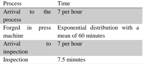
The data analysed are provided by the same problem, which can be seen in table 1, which specifies times of each process, as well as arrivals. Times for some events are defined by probability distributions, it is also mentioned that arrivals are metal parts, that when passing through the press end as wings, then they pass to the inspection area to finally leave the process.

Table 1. Collection of data of process times.

Process Time

Arrival to the process

7 per hour

Forged in press machine

Exponential distribution with a mean of 60 minutes

Arrival to

inspection

7 per hour

Inspection 7.5 minutes

As part of the data provided of the problem, below is the values with which the process can work; power of the press with its times and respective cost per hour; the type of inspector is to say that an inspector can be used who does his work in 7.2 minutes or another who does it in 7.5 minutes, each with a different cost per hour.

A= Power of the press

• low level E (48) minutes cost = $7.50 per hour • Intermediate level E (60) minutes cost=$7.00 per hour • High level E (72) minutes cost=$6.50 per hour B=Inspector

• low level 7.2 minutes cost=$19.00 per hour • High level 7.5 minutes cost=$17.00 per hour

D. Implementation Of The Model On Computer

630

Rafael Bello Morales

, ETJ

Volume 4 Issue 09 September 2019

E. Validation Of The Model

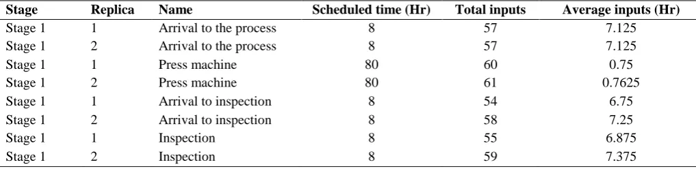
According to Herrera & Becerra 15, the method of future prediction is a method used to validate simulation processes, which was applied to analyse the data of arrivals of the real system of the problem of Table 1 in contrast to the average of two replicates of entries per hour of the proposed model of table 2.

Because it is a problem that was obtained from the specialized literature, it was ensured that the entries in the model coincided with the entries of the proposed model, in addition to the construction of entities, locations, arrivals and the process as specified in the problem. When the model was run there were no complications in terms of routing or failed arrivals, which is important to be able to collect results that help with the analysis. With this, it is possible to say that there is no significant difference between the values obtained from the simulation and the actual values provided.

Table 2. Arrivals to the simulated system process.

F. Experimentation

Once the model is constructed it is necessary to plan the experiments based on the levels of each factor as shown in table 2, the design is factorial with mixed levels because the factor of inspection is at two levels and the speed of the press machine is at three levels as shown in the collection of data, power of the press expressed with the letter "A" has

three levels: low, intermediate and high, which refers to the speed with which the press can work. Therefore, it is said that it is a 3 X 2 factorial design with mixed levels with 6 treatments, to have better results, two replicas are proposed, so there will be 12 experimental runs, in addition to helping to obtain greater degrees of freedom for the error and get a more accurate result.

Table 3. Notation of treatments.

G. INTERPRETATION OF RESULTS

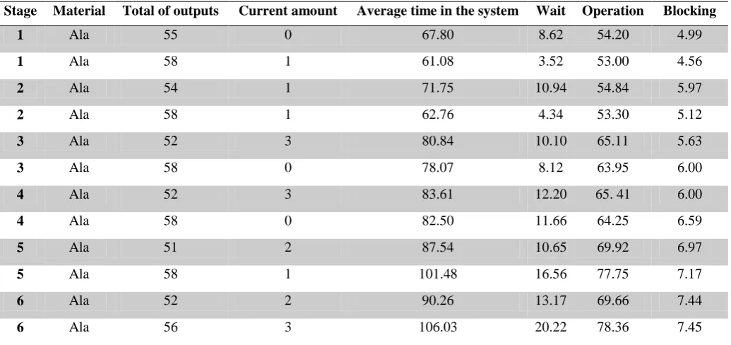
Once the scenarios were simulated, the data collected by ProModel software was collected as shown in table 4, which shows results of simulation and replication of each scenario during a period of 8 hours. It contains total of outputs, amount of current material (current wing inventory), as well

as average time in the system that is given by the sum of the waiting time, time in operation and time of block.

The main objective of this research focuses on optimizing the work in process while reducing the production cost, so it seeks to optimize the quantities of inventory before each work station so as to minimize the waiting time of unprocessed wings. Time in the system is given by the sum

Stage Replica Name Scheduled time (Hr) Total inputs Average inputs (Hr)

Stage 1 1 Arrival to the process 8 57 7.125

Stage 1 2 Arrival to the process 8 57 7.125

Stage 1 1 Press machine 80 60 0.75

Stage 1 2 Press machine 80 61 0.7625

Stage 1 1 Arrival to inspection 8 54 6.75

Stage 1 2 Arrival to inspection 8 58 7.25

Stage 1 1 Inspection 8 55 6.875

Stage 1 2 Inspection 8 59 7.375

Treatment combination Real treatment

Corrida A B A B Press time (A) Inspection time (B)

1 -1 -1 Low low 48 min 7.2 min

2 -1 +1 Low High 48 min 7.5 min

3 0 -1 Intermediate low 60 min 7.2 min

4 0 +1 Intermediate High 60 min 7.5 min

5 +1 -1 High low 72 min 7.2 min

631

Rafael Bello Morales

, ETJ

Volume 4 Issue 09 September 2019

of wait, operation and blockage as shown in table 4, by reducing these indicators will help meet the objective of

minimizing work in process and minimizing cost of production.

Table 2. Work in process time in the system.

Stage Material Total of outputs Current amount Average time in the system Wait Operation Blocking

1 Ala 55 0 67.80 8.62 54.20 4.99

1 Ala 58 1 61.08 3.52 53.00 4.56

2 Ala 54 1 71.75 10.94 54.84 5.97

2 Ala 58 1 62.76 4.34 53.30 5.12

3 Ala 52 3 80.84 10.10 65.11 5.63

3 Ala 58 0 78.07 8.12 63.95 6.00

4 Ala 52 3 83.61 12.20 65. 41 6.00

4 Ala 58 0 82.50 11.66 64.25 6.59

5 Ala 51 2 87.54 10.65 69.92 6.97

5 Ala 58 1 101.48 16.56 77.75 7.17

6 Ala 52 2 90.26 13.17 69.66 7.44

6 Ala 56 3 106.03 20.22 78.36 7.45

As mentioned earlier, because the objective is to optimize the work in process and total cost of production, costs of work in process per hour and costs of using different inspector were considered; as well as cost of working with the press to different levels. The costs are specified in table 5.

Table 5. Process costs.

Costs

WIP cost per hour $8

Power Press (A)

Low $7.5

Intermediate $7

High $6.5

Inspection (B)

Low $19

High $17

With help of table 4 and 5, the cost equations were presented to obtain the values of the output response for an 8-hour per day. Equation 1 represents the cost of work in process.

Equation 2 represents the cost of labour where the cost of inspection and the press are multiplied by 8, due to the total hours of the workday that is analysed. In equation 3 the total cost of production is represented, which expresses the sum of labour and WIP costs.

t*(r+s)*x=u (1)

z*8+y*8=v (2)

u+v=w (3)

Where:

r= Total outputs w= Total production cost s= Current amount of material x= WIP cost per hour t= Average time in the system y= Cost per press level u= WIP cost z= Inspection cost v= Workforce cost

The results obtained from the simulation were converted to costs by means of equations 1,2 and 3 given in table 6, where response variables "WIP cost" and "Total production cost" can be observed that will be analysed by design of experiments. Regarding "Workforce cost" column, it was used to generate the "total production cost".

Table 6. WIP cost, Workforce cost and production cost per scenario.

Stage WIP cost ($) Workforce cost ($) Total production cost ($)

1 497.2 212 709.2

2 526.166 196 722.166

3 592.826 208 800.826

4 613.14 192 805.14

5 618.616 204 822.616

632

Rafael Bello Morales

, ETJ

Volume 4 Issue 09 September 2019

7 480.496 212 692.496

8 493.712 196 689.712

9 603.741 208 811.741

10 638.00 192 830.00

11 798.309 204 1002.309

12 834.102 188 1022.102

Once the results were obtained it is important to make sure that these are useful for design of experiments. Statistical methods were used to analyse the data, ensuring that results and conclusions were objective 7. Due to this it will be necessary to apply a normality assumption to the response variables according to Garza 16 and Pérez, Arango & Agudelo 17 where the rule of normality assumption is that if p-value is greater than 0.05 with a confidence level of 95%, then the data is normal. In this case it can be seen in figures 3 and 4 that there is a p-value of 0.133 and 0.059, respectively, which confirms that the data is within the normal range.

Figure 3. WIP cost probability plot.

Figure 3. Total production cost probability plot.

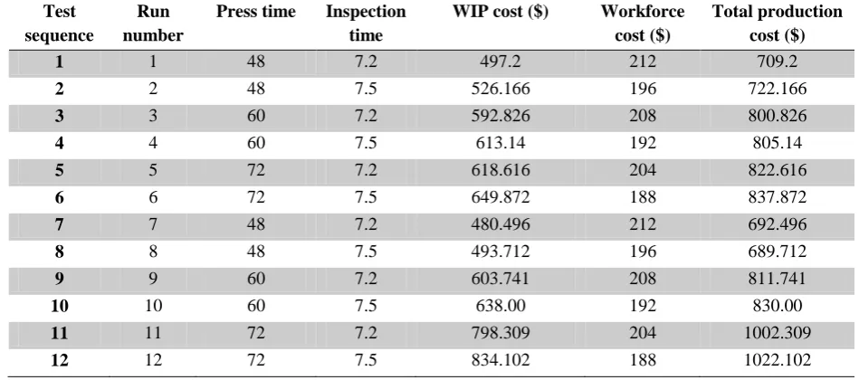
Once the data was obtained and its normality confirmed, MINITAB software was used as a tool to apply design of experiments. When analysing a factorial design with mixed levels it was necessary to enter it as a general complete factorial design with 2 factors, where press time takes three levels (48 min, 60 min, 72 min) and inspection time at two levels (7.2 min, 7.5 min), remembered that 2 replicas are considered. Table 7 shows the complete factorial design that was analysed by the software.

Table 7. Complete factorial design of the experiment.

Test sequence

Run number

Press time Inspection time

WIP cost ($) Workforce cost ($)

Total production cost ($)

1 1 48 7.2 497.2 212 709.2

2 2 48 7.5 526.166 196 722.166

3 3 60 7.2 592.826 208 800.826

4 4 60 7.5 613.14 192 805.14

5 5 72 7.2 618.616 204 822.616

6 6 72 7.5 649.872 188 837.872

7 7 48 7.2 480.496 212 692.496

8 8 48 7.5 493.712 196 689.712

9 9 60 7.2 603.741 208 811.741

10 10 60 7.5 638.00 192 830.00

11 11 72 7.2 798.309 204 1002.309

12 12 72 7.5 834.102 188 1022.102

Analysis of variance (ANOVA) helps to identify the importance of each factor and interactions through the effects of each of the variables, which can define which

633

Rafael Bello Morales

, ETJ

Volume 4 Issue 09 September 2019

We analysed the p-value considered a confidence level of 95%, so that a value of P less than 0.05 means that this factor is important for the model. Considering 95% confidence level in table 8, it can be concluded that the only

significant value in the model is press time. Table 8 also shows that R2 = 75.34% refers to the significant factors within the ANOVA explain the model in 75.34%.

Table 8. ANOVA of WIP cost.

factor GL SC Adjust. MC Adjust. Valour F Valour p

Model 5 104313 20862.6 3.67 0.073

Linear 3 104236 34745.3 6.10 0.030

Press time 2 102000 51000.0 8.96 0.016

Inspection time 1 2236 2236.0 0.39 0.554

Interactions of 2 terms 2 77 38.6 0.01 0.993

Press time * Inspection time 2 77 38.6 0.01 0.993

Error 6 34150 5691.7

Total 11 138463

S= 75.4432 R2 = 75.34% R2 adj= 54.78% R2 pred= 1.35%

When analysing the ANOVA of the total production cost in table 9 it can be said that the value with the greatest effect is the time of the press when presenting the highest value of the effects, in addition P value was analysed in which it is noted that the only significant value within the model for the

total production cost is the time of the press to be a value less than 0.05 depending on the level of reliability used. Table 9 shows that R2 = 73.63% that refers to the significant factors within the ANOVA explain the model in 73.63%.

Table 9. ANOVA of total production cost.

factor GL SC Adjust. MC Adjust. Valour F Valour p

Model 5 95362 19072.4 3.35 0.087

Linear 3 95284 31761.5 5.58 0.036

Press time 2 94901 47450.7 8.34 0.019

Inspection time 1 383 383.1 0.07 0.804

Interactions of 2 terms 2 77 38.6 0.01 0.993

Press time * Inspection time 2 77 38.6 0.01 0.993

Error 6 34150 5691.7

Total 11 129512

S= 75.4432 R2 = 73.63% R2 adj= 51.66% R2 pred= 0.00%

H. OPTIMIZATION OF THE MODEL

For the optimization part, MATLAB software tools "response optimizer" was obtained, obtaining the results of figure 5 where it can be seen that the model is optimized by having press time in 48 min and inspection time in 7.2 min., with which “WIP cost” output response has an average minimum cost of $ 488.8480 per day and the response variable "total production cost" has an average minimum cost of $ 700.8480 per day.

634

Rafael Bello Morales

, ETJ

Volume 4 Issue 09 September 2019

Based on the results obtained with the methodology proposed in the research, it can be said that the current process in Table 1, if we want to improve it in the real system, it is necessary to make changes in the press times and the time of the inspector to obtain a better process efficiency as specified in the optimization part. Because it has been proven by the design of experiments to confirm the levels with which it must work and what is the critical point of the model.

IV. CONCLUSIONS

The series of steps applied in the methodology developed through the design of experiments and discrete simulation facilitated the elaboration and analysis of the model, as well as the obtaining and analysis of the final results, with which it can be said that the methodology used in this article was able to reduce the work in process and consequently the cost of WIP and the total production cost.

The use of discrete simulation using ProModel software was a fundamental part of the research, helping to build the computer model and obtaining the output responses that were used to analyse the design of experiments.

The MINITAB software application was necessary to apply statistical tests and perform the design of experiments to facilitate the ANOVA analysis, in which factors A (press time), B (inspection time) and AB interaction were added. Results were obtained with which it can be concluded that the only significant value in the process is the press time, when analysed with a confidence level (p-value) of 95% and that the only value below .05 within the ANOVA.

It can be concluded that the methodology used was able to fulfil the objective of optimizing the work in process, with simulation and the results of table 4 it is observed that the time of work in process given by the waiting times, operation and blocking of the scenario 1 and its replication become smaller than in scenarios 2,3,4,5 and 6, due to this in table 6 it can be seen that according to the times it is how the cost of WIP increases and the total production cost. It was possible to optimize the WIP costs and the total production costs by knowing the levels of each factor, where press time must be 48 minutes and inspection time must be 7.2 minutes. The factor with the greatest impact for the work in process and costs, is the press time with which it can be said that in the case of wanting to further reduce the work in process and the costs the first thing that should be done is decrease press time.

BIBLIOGRAPHY

1. Valenzuela, J. & Palacios, J. Reducir el tiempo de preparaciónutilizando el sistema SMED en una máquina de producción por medio de la metodológia DMAIC. in IngenieriaVertice 2010 13–24 (2014).

2. Sanchez, P. A., Ceballos, F. & Torres, G. S. A

dressmaking factory production process analysis modeling and simulation. Cienc. e Ing. Neogranadina 25, 137–150 (2015).

3. Blanco, L. E., Romero, E. &Páez, J. A. Conwip un sistema de control de producción. Fourth LACCEI Int. Lat. Am. Caribb. Conf. Eng. Technol. 21–27 (2006).

4. Dinas, J. A., Franco, P. & Rivera, L. A. Aplicación de herramientas de pensamientosistémico para el aprendizaje de Lean Manufacturing. Sist. Telemat. 7, 109–144 (2009).

5. Sundar, R., Balaji, A. N. &SatheeshKumar, R. M. A review on lean manufacturing implementation techniques. Procedia Eng. 97, 1875–1885 (2014). 6. García, E., García, H. & Cárdenas, L. E.

Simulación y análisis de sistemas con ProModel. (Pearson Educación de México, S.A. de C.V., 2013).

7. Ilzarbe, L., Tanco, M., Viles, E. & Álvarez, M. J. El diseño de experimentoscomoherramienta para la mejora de los procesos. Aplicación de la metodología al caso de una catapulta. Tecnura 10, 127–138 (2007).

8. Ceballos, J. A., Restrepo, E. D. & Fernández, J. D. Aplicación De Un Modelo De Simulación DiscretaEn El Sector Del ServicioAutomotor. Rev. Ing. Ind. UPB 01, 51–61 (2013).

9. Pergher, I. & Vaccaro, G. L. R. Work in process level definition: a method based on computer simulation and electre tri. Production 24, 536–547 (2013).

10. Jayaprakash, J., Kumar, K. M. & Ambedkar, P. Simulation of Mixed Model Assembly Line Sequencing Using Pro-Model Software. Int. J. Appl. Eng. Res. 10, 854–856 (2015).

11. Bernal, M. E., Cock, G. &Rastrepo, J. H. Productividaden una celda de manufactura flexible simuladaenpromodelutilizando path networks type crane. Tectura 19, 133–144 (2015).

12. Coss, R. Simulación un enfoquepráctico. (Limusa Noriega Editores, 2002).

13. Menéndez, G., Bonavetti, V. L. &Irassar, E. F. Los Diseños de Experimentos y la Tecnología del Hormigón. Rev. la Construcción 7, 94–104 (2008). 14. Hillier, F. S. & Lieberman, G. J. Introduccón a la

investigacíon de operaciones. 3, (The McGraw-Hill Companies, Inc, 2010).

15. Herrera, O. J. & Becerra, L. A. Diseño general de las etapas de simulación de procesos con énfasisen el análisis de entrada. in Twelfth LACCEI Latin American and Caribbean Conference for Engineering and Technology 10 (Excellence in Engineering To Enhance a Country’s Productivity, 2014).

635

Rafael Bello Morales

, ETJ

Volume 4 Issue 09 September 2019

para el analisis de secado de un producto (Experiment design application for analysis of the drying a product). Innovaciones de Negocios 10, 145–158 (2013).

17. Pérez, G., Arango, M. D. &Agudelo, Y. Aplicación del diseño de experimentos para el análisis del proceso de doblado. Rev. EIA 11, 145–156 (2009). 18. Ekren, B. Y. &Ornek, A. M. A simulation based

experimental design to analyze factors affecting production flow time. Simul. Model. Pract. Theory 16, 278–293 (2008).