Flows
By MICHAELW. L. ELSBY ANDRYANMICHAELS
This paper introduces a notion of firm size into a search and match-ing model with endogenous job destruction. The outcome is a rich, yet analytically-tractable framework that can be used to analyze a broad set of features of both the cross-section and aggregate dynamics of the labor market. The model provides a coherent account of a) the distributions of employer size and employment growth across establishments; b) the amplitude and propagation of cyclical fluctuations in worker flows; c) the negative comovement of unemployment and vacancies; and d) the dynamics of the distribution of employer size over the business cycle.
The study of the macroeconomics of labor markets has been dominated by two influ-ential approaches in recent research: the development of search and matching models (Pissarides 1985; Mortensen and Pissarides 1994) and the empirical analysis of estab-lishment dynamics (Davis and Haltiwanger 1992). This paper provides an analytical framework that unifies these approaches by introducing a notion of firm size into a search and matching model with endogenous job destruction. The outcome is a rich, yet analytically-tractable framework that can be used to analyze a broad set of features of both the cross section and the dynamics of the aggregate labor market. In a set of quantitative applications we show that the model can provide a coherent account of a) the salient features of the distributions of employer size, and employment growth across establishments; b) the amplitude and propagation of cyclical fluctuations in flows be-tween employment and unemployment; c) the negative comovement of unemployment and vacancies in the form of the Beveridge curve; and d) the dynamics of the distribution of employer size over the business cycle.
A notion of firm size is introduced by relaxing the common assumption that firms face a linear production technology.1 Though conceptually simple, incorporating this feature is not a trivial exercise. The existence of a nonlinear production technology, Elsby: School of Economics, University of Edinburgh, 31 Buccleuch Place, Edinburgh, EH8 9JT, United Kingdom, [email protected]. Michaels: Department of Economics, University of Rochester, 234 Harkness Hall, Rochester, NY 14627, [email protected]. We are grateful to Gary Solon and Matthew Shapiro for their comments, support, and encouragement, to numerous anonymous referees for very constructive comments, and to John Haltiwanger, Ron Jarmin, and Javier Miranda for providing us with tabulations from the Longitudinal Business Database. We also thank Mark Bils, Björn Brügemann, Shigeru Fujita, William Hawkins, Bart Hobijn, Oleg Itskhoki, Winfried Koeniger, Per Krusell, Toshi Mukoyama, Ay¸segül ¸Sahin, Dmitriy Stolyarov, and Marcelo Veracierto for helpful discussions as well as seminar participants at the May 2007 UM/MSU/UWO Labor Day, the European Central Bank, the Kansas City Fed, UQAM, the NewYork/Philadelphia Fed Workshop on Quantitative Macroeconomics, Yale, the 2008 CEPR ESSLE con-ference, the Minneapolis Fed, Chicago Booth, Oslo, Oxford, Edinburgh and the 2012 American Economic Association Meetings for helpful comments. In addition, we are grateful to William Hawkins for catching a coding error in an earlier draft of this paper. All remaining errors are our own.
1In its simplest form, this manifests itself in a one-firm, one-job representation, as in Pissarides (1985) and Mortensen
and Pissarides (1994).
and the associated presence of multi-worker firms, complicates wage setting because the surplus generated by each of the employment relationships within a firm is not the same—“the” marginal worker generates less surplus than infra-marginal workers. In section 1, we apply the bargaining solution of Stole and Zwiebel (1996) to derive a very intuitive wage bargaining solution for this environment, something that has been considered challenging in recent research (see Cooper, Haltiwanger and Willis 2007, and Hobijn and ¸Sahin forthcoming). The solution is a very natural generalization of the wage bargaining solution in standard search and matching models. The simplicity of our solution is therefore a useful addition to the literature.2
The wage bargaining solution enables us to characterize the properties of the optimal labor demand policy of an individual firm in the presence of idiosyncratic firm hetero-geneity. We demonstrate that the labor demand solution is analogous to that of a model of kinked hiring costs in the spirit of Bentolila and Bertola (1990), but where the hiring cost is endogenously determined by frictions in the labor market. This yields an analyti-cal solution for the optimal labor demand policy, summarizing microeconomic behavior in the model.
In section 2, we take on the task of aggregating this behavior to the macroeconomic level. This is a challenge because the presence of a nonlinear production technology and idiosyncratic heterogeneity imply that a representative firm interpretation of the model does not exist. To address this, we develop a method that allows us to solve analytically for the equilibrium distribution of employment across firms (the firm size distribution). In turn, this allows us to determine the level of the aggregate (un)employment stock, which is implied by the mean of that distribution. We also provide a related method that allows us to solve for aggregate unemployment flows (hires and separations) implied by microeconomic behavior. Together, these characterize the aggregate steady-state equi-librium of the model economy.
In section 3 we explore the dynamics of the model by introducing aggregate shocks. A difficulty that arises in the model is that, out of steady state, individual firms must forecast future wages, which involves forecasting the future path of the distribution of employment across firms, an infinite-order state variable. A useful feature of our analyti-cal solution for optimal labor demand is that it allows us to simplify part of this problem. In particular, we are able to derive an analytical approximation to a firm’s optimal labor demand policy in the presence of aggregate shocks, obviating the need for a numeri-cal solution. Using this, we employ an approach that mirrors the method proposed by Krusell and Smith (1998) to solve for the transition paths for the unemployment stock and flows in the presence of aggregate shocks.
These results form the basis of a series of quantitative applications, which we turn to
2Bertola and Caballero (1994) solve a related bargaining problem by taking a linear approximation to the marginal
in section 4. An attractive feature of the model is that, by incorporating both a notion of firm size as well as idiosyncratic heterogeneity, it delivers important cross-sectional im-plications.3 We show that the model can be used to match key features of the distribution of firm size, and of employment growth across establishments. This is achieved through two aspects of the model. First, due to the existence of kinked hiring costs, optimal la-bor demand features a region of inaction whereby firms choose neither to hire nor fire workers. This matches a key property of the distribution of employment growth—the existence of a mass point at zero establishment growth—noted at least since the work of Davis and Haltiwanger (1992).4Second, informed by the well-known shape of the distri-bution of firm size, we adopt a Pareto specification for idiosyncratic firm productivity. A surprising outcome of this approach is that the Pareto specification also provides a very accurate description of the tails of the distribution of employment growth, something that cannot be achieved using more conventional lognormal specifications of heterogeneity.
We then use these steady-state features of the model to provide a novel perspective on the cyclical dynamics of worker flows implied by the model. It is well-known that the cyclical amplitude of unemployment, and of the job-finding rate in particular, relies critically on the size of the surplus to employment relationships (Shimer 2005; Hagedorn and Manovskii 2008). Intuitively, small reductions in aggregate productivity can easily exhaust a small surplus, and lead firms to cut back substantially on hiring. The presence of large and heterogeneous firms in our model opens up a new approach to calibrating the payoff from unemployment, and thereby the match surplus. Because the model is capable of matching the observed cross-sectional distribution of employment growth, we obtain a sense of the plausible size of idiosyncratic shocks facing firms. Given this, a higher payoff from unemployment implies a smaller surplus, so that jobs will be destroyed more frequently, raising the rate of worker turnover. We discipline the model by choosing the payoff from unemployment that matches the empirical rate at which employed workers flow into unemployment.
Applying this approach to an otherwise standard calibration reveals that our gener-alized model can replicate both the observed procyclicality of the job-finding rate, as well as the countercyclicality of the employment-to-unemployment transition rate in the U.S.5We show that this is a substantial improvement over standard search and matching models. As shown by Shimer (2005), these are unable to generate enough cyclicality in job creation. To overcome this, the standard model must reduce the size of the surplus, which in turn yields excessive employment-to-unemployment transitions.6 The
general-3In terms of its implications for cross-sectional establishment dynamics, the model shares many of the features of
the seminal work of Hopenhayn and Rogerson (1993). We show that these cross-sectional features are very useful for disciplining aspects of the model driven by search frictions, notably the magnitude of the average surplus to employment relationships, which are crucial for the aggregate implications of models with matching frictions.
4Earlier work by Hamermesh (1989), which analyzed data from seven manufacturing plants, also drew attention to
the “lumpy” nature of establishment-level employment adjustment.
5For evidence on the countercyclicality of employment-to-unemployment flows, see Perry (1972); Marston (1976);
Blanchard and Diamond (1990); Elsby, Michaels, and Solon (2009); Fujita and Ramey (2009); Pissarides (2007); Shimer (2012); and Yashiv (2007).
6This formalizes the intuition of recent research that has argued that the average surplus required for the standard
ized model does not face this tension between reproducing the cyclicality of job creation and the rate of worker turnover. Due to the diminishing marginal product of labor, the model generates simultaneously a large average surplus and a small marginal surplus to employment relationships. The former allows the model to match the rate at which workers flow into unemployment, the latter the volatility of the job-finding rate over the cycle.7
A potential concern in models that incorporate countercyclical job destruction, such as the model in this paper, has been that they often cannot generate the observed procycli-cality of vacancies (Shimer 2005; Mortensen and Nagypal 2008). Importantly, we find that our model makes considerable progress in this regard: Our calibration of the model generates most of the observed comovement between vacancies and output per worker. As a result, it reproduces a key stylized fact of the U.S. labor market: the negative co-movement between unemployment and vacancies in the form of the Beveridge curve. The model therefore provides a coherent and quantitatively accurate picture of the joint cyclical properties of both flows of workers in and out of unemployment, as well as the behavior of unemployment and vacancies.
A less well-documented limitation of the standard search and matching model relates to the propagation of the response of the job-finding rate to aggregate shocks to labor productivity. The job-finding rate is a jump variable in the standard model, responding instantaneously to aggregate shocks, while it exhibits a sluggish response in U.S. data. An appealing feature of the generalized model is that it delivers a natural propagation mechanism: The job-finding rate is a function of the distribution of employment across firms, which we show is a slow-moving state variable in our model. Simulations reveal that this aspect of the model can help account for the persistence of the decline in job creation following an adverse shock.
Our efforts to understand the amplification and propagation of labor market flows over the business cycle are related to the important early work of Cooper, Haltiwanger, and Willis (2007). They also study a random matching model with decreasing returns. This paper’s model differs from theirs in at least two regards. First, Cooper et al. suppress worker bargaining power. This simplifies wage bargaining, but at the cost of severing the link between the bargained wage, on the one hand, and market tightness on the other. This paper investigates a more general bargaining rule that allows workers to extract some of the rents. Second, Cooper et al. include additional labor market frictions, such as fixed costs to hire and fire. We agree that the interaction of these adjustment costs with matching frictions deserves further attention. However, we find it helpful to abstract from these for a number of reasons. In particular, we are able to make substantial headway in characterizing the analytics of optimal establishment-level labor demand and aggregate job creation. This in turn allows us to highlight the effects of decreasing returns and to U.S. economy, which researchers have taken to imply substantial rents to ongoing matches (Hall 1982; Stevens 2005).
7One might imagine that a symmetric logic holds on the supply side of the labor market if there is heterogeneity
contrast our model more tightly with that in Mortensen and Pissarides. Thus, we see our paper as complementary to Cooper et al., who study a richer model but rely principally on numerical solution methods.
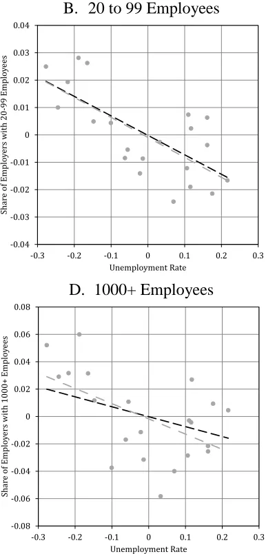
In the closing sections of the paper, we move beyond characterizing the business cycle properties of the model and turn to evaluating its implications for a number of additional cross-sectional outcomes. First, recent literature has emphasized empirical regularities in the cyclical behavior of the cross-sectional distribution of establishment size: While the share of small establishments with fewer than 20 workers rises during recessions, the shares of larger firms decline (Moscarini and Postel-Vinay 2008). The model replicates this observation: For each establishment size class considered, it broadly matches the comovement with unemployment over the business cycle observed in U.S. data. Given that these implications of the model are venturing farther afield from the moments it was calibrated to match, we view these results as an important achievement.
In our final quantitative application, we evaluate the model’s ability to account for the observation that workers employed in larger firms are often paid higher wages— the employer size-wage effect (Brown and Medoff 1989). A distinctive attribute of the model is that, by incorporating large firms with heterogeneous productivities, it can speak to this empirical regularity. The magnitude of the size-wage effect implied by the model is mediated by two competing forces, as noted by Bertola and Garibaldi (2001). On the one hand, the existence of diminishing returns in production might lead one to anticipate a negative relation between employer size and wages. On the other, larger firms also tend to be more productive. Quantitatively, the latter dominates, generating one quarter of the empirical size-wage effect.
The remainder of the paper is organized as follows. Section 1 describes the set-up of the model, and characterizes the wage bargaining solution together with the associated optimal labor demand policy of an individual firm. Given this, section 2 develops a method for aggregating this microeconomic behavior up to the macroeconomic level, and uses it to characterize the steady state equilibrium of the model. Section 3 introduces aggregate shocks to the analysis. It presents an approach to computing the out of steady state dynamics of the model through the use of analytical approximations. We then use the model in section 4 to address a wide range of quantitative applications. Finally, section 5 summarizes our results, and draws lessons for future research.
I. The Firm’s Problem
of average net job creation, their contribution to the cyclicality of aggregate employment growth is small. In section 5, we return to the issue of entry in a more extended discussion of the recent literature.
In order to hire unemployed workers, firms must post vacancies. However, frictions in the labor market limit the rate at which unemployed workers and hiring firms can meet. As is conventional in the search and matching literature, these frictions are embodied in a matching function, M D M.U;V/, that regulates the number of hires, M, that the economy can sustain given that there are V vacancies and U unemployed workers. We assume that M.U;V/exhibits constant returns to scale.8 Vacancies posted by firms are therefore filled with probability q D M=V D M.U=V;1/each period. Likewise, un-employed workers find jobs with probability f D M=U DM.1;V=U/. Thus, the ratio of aggregate vacancies to aggregate unemployment, V=U , is a sufficient statistic for the job filling (q) and job finding ( f ) probabilities in the model. Taking these flow probabilities as given, firms choose their optimal level of employment, to which we now turn.
A. Labor Demand
We consider a discrete-time, infinite-horizon model in which firms use labor, n, to produce output according to the production function, y D px F.n/where F0 > 0 and F00 0. The latter is a key generalization of the standard search model that we consider:
When F00 < 0, the marginal product of labor will decline with firm employment, and
thereby will generate a downward-sloped demand for labor at the firm level. p represents the state of aggregate labor demand, whereas x represents shocks that are idiosyncratic to an individual firm. We assume that the evolution of the latter idiosyncratic shocks is described by the c.d.f. G x0jx .
A typical firm’s decision problem is completely analogous to that in Mortensen and Pissarides (1994), and is as follows. Firms observe the realization of their idiosyncratic shock, x, at the beginning of a period. Given this, they then make their employment decision. Specifically, they may choose to separate from part or all of their workforce, which we assume may be done at zero cost. Any such separated workers then join the unemployment pool in the subsequent period. Alternatively, firms may hire workers by posting vacancies,v 0, at a flow cost of c per vacancy. If a firm posts vacancies, the matching process then matches these up with unemployed workers inherited from the previous period. After the matching process is complete, production and wage setting are performed simultaneously.
It follows that we can characterize the expected present discounted value of a firm’s profits,5 .n 1;x/, recursively as:9
8See Petrongolo and Pissarides (2001) for a summary of empirical evidence that suggests this is reasonable. 9We adopt the convention of denoting lagged values with a subscript,
(1) 5 .n 1;x/Dmax
n;v px F.n/ w .n;x/n cvC Z
5 n;x0 d G x0jx ;
wherew .n;x/is the bargained wage in a firm of size n and productivity x. A typical firm seeks a level of employment that maximizes its profits subject to a dynamic constraint on the evolution of a firm’s employment level. Specifically, firms face frictions that limit the rate at which vacancies may be filled: A vacancy posted in a given period will be filled with probability q <1 prior to production. Thus, the number of hires an individual firm achieves is given by:
(2) 1n1C Dqv;
where1n is the change in employment, and 1Cis an indicator that equals one when the
firm is hiring, and zero otherwise. Substituting the constraint, (2), into the firm’s value function, we obtain:10
(3) 5 .n 1;x/Dmax
n px F.n/ w .n;x/n
c q1n1
CC Z
5 n;x0 d G :
Note that the value function is not fully differentiable in n: There is a kink in the value function around n D n 1.11 This reflects the (partial) irreversibility of separation deci-sions in the model. While firms can shed workers costlessly, it is costly to reverse such a decision because hiring (posting vacancies) is costly. In this sense, the labor demand side is formally analogous to the kinked employment adjustment cost model of the form analyzed in Bentolila and Bertola (1990), except that the per-worker hiring cost, c=q. /, is endogenously determined.12
In order to determine the firm’s optimal employment policy, we take the first-order conditions for hires and separations (i.e. conditional on1n 6D0):
(4) px F0.n/ w .n;x/ w
n.n;x/n
c q1
CC D.n;x/D0, if1n 6D0;
where D.n;x/ R 5n n;x0 d G x0jx reflects the marginal effect of current employ-ment decisions on the future value of the firm. Equation (4) is quite intuitive. It states
10Henceforth, “d G” without further elaboration is to be taken to mean “d G x0jx ”.
11An implicit assumption is that there are no exogenous quits in the model. Fujita and Nakajima (2009) have analyzed
an extension of our model that includes exogenous quits, with very similar results.
12A drawback of the kinked adjustment cost structure implied by the model is that it is inconsistent with evidence on
that the marginal product of labor ( px F0.n/) net of any hiring costs (c
q1C), plus the dis-counted expected future marginal benefits from an additional unit of labor ( D.n;x/) must equal the marginal cost of labor (w .n;x/Cwn.n;x/n). To provide a full charac-terization of the firm’s optimal employment policy, it remains to characterize the future marginal benefits from current employment decisions, D.n;x/, and the wage bargaining solution,w .n;x/, to which we now turn.
B. Wage Setting
The existence of frictions in the labor market implies that it is costly for firms and workers to find alternative employment relationships. As a result, there exist quasi-rents over which the firm and its workers must bargain. The assumption of constant marginal product in the standard search model has the tractable implication that these rents are the same for all workers within a given firm. It follows that firms can bargain with each of their workers independently, because the rents of each individual employment relationship are independent of the rents of all other employment relationships.
Allowing for the possibility of diminishing marginal product of labor F00.n/ < 0,
however, implies that these rents will depend on the number of workers within a firm. Intuitively, the rent that a firm obtains from “the” marginal worker will be lower than the rent obtained on all infra-marginal hires due to diminishing marginal product. An implication of the latter is that the multilateral dimension of the firm’s bargain with its many workers becomes important: The rents of each individual employment relationship within a firm are no longer independent.
To take this into account, we adopt the bargaining solution of Stole and Zwiebel (1996) which generalizes the Nash solution to a setting with diminishing returns.13 Stole and Zwiebel present a game where the bargained wage is the same as the outcome of simple Nash bargaining over the marginal surplus. The game that supports this simple result is one in which a firm negotiates with each of its workers in turn, and where the breakdown of a negotiation with any individual worker leads to the renegotiation of wages with all remaining workers.14
The empirical validity of the Stole and Zwiebel bargaining solution has yet to be as-sessed. Instead, our motivation for using the Stole and Zwiebel protocol is to keep the behavior of wages as close to that implied by the standard search model, in order to draw out the implications of decreasing returns. We will see in what follows that the bargaining solution implied by the Stole and Zwiebel protocol is helpful in this regard, since it bears a strong resemblance to the Nash bargaining solution in the Mortensen and Pissarides (1994) model.
13This approach was first used by Cahuc and Wasmer (2001) to generate a wage equation for the exogenous job
destruction case.
14The intuition for the Stole and Zwiebel result is as follows. If the firm has only one worker, the firm and worker
In accordance with the timing of decisions each period, wages are set after employment has been determined. Thus, hiring costs are sunk at the time of wage setting, and the marginal surplus, which we denote as J.n;x/, is equal to the marginal value of labor gross of the costs of hiring:
(5) J.n;x/D px F0.n/ w .n;x/ w
n.n;x/nC D.n;x/ :
The surplus from an employment relationship for a worker is the additional utility a worker obtains from working in her current firm over and above the utility she obtains from unemployment. The value of employment in a firm of size n and productivity x,
W.n;x/, is given by:
(6) W.n;x/Dw .n;x/C E s70C.1 s/W n0;x0 jn;x :
While employed, a worker receives a flow payoff equal to the bargained wage,w .n;x/. She loses her job with (endogenous) probability s next period, upon which she flows into the unemployment pool and obtains the value of unemployment,70. With probability
.1 s/, she retains her job and obtains the expected payoff of continued employment in her current firm, W n0;x0 . Likewise, the value of unemployment to a worker is given
by:
(7) 7 DbC E .1 f/ 70C f W n0;x0 :
Unemployed workers receive flow payoff b, which represents unemployment benefits and/or the value of leisure to a worker. They find a job next period with probability f , upon which they obtain the expected payoff from employment, W n0;x0 .
Wages are then the outcome of a Nash bargain between a firm and its workers over the marginal surplus, with worker bargaining power denoted as :
(8) .1 /[W.n;x/ 7]D J.n;x/ :
Given this, we are able to derive a wage bargaining solution with the following simple structure:
PROPOSITION 1: The bargained wage,w .n;x/, solves the differential equation15
(9) w .n;x/D px F0.n/ w
n.n;x/nC f
c
q C.1 /b:
The intuition for (9) is quite straightforward. As in the standard search model, wages are increasing in the worker’s bargaining power, , the marginal product of labor, px F0.n/,
15This solution extends the solution obtained by Cahuc and Wasmer (2001) to the case with endogenous job
workers’ job finding probability, f , the marginal costs of hiring for a firm, c=q, and
workers’ flow value of leisure, b. There is an additional term, however, inwn.n;x/n. To understand the intuition for this term, consider a firm’s negotiations with a given worker. If these negotiations break down, the firm will have to pay its remaining workers a higher wage. The reason is that fewer workers imply that the marginal product of labor will be higher in the firm, which will partially spillover into higher wages (wnn < 0). The more powerful this effect is (the more negative iswnn), the more the firm loses from a given breakdown of negotiations with a worker, and the more workers can extract a higher wage from the bargain.
In what follows, we will adopt the simple assumption that the production function is of the Cobb-Douglas form, F.n/Dn with 1. Given this, the differential equation for the wage function, (9), has the following simple solution:16
(10) w .n;x/D px n
1
1 .1 / C f
c
q C.1 /b:
Setting D1 yields the discrete time analogue to the familiar wage bargaining solution for the Mortensen and Pissarides (1994) model.
C. The Firm’s Optimal Employment Policy
Now that we have obtained a solution for the bargained wage at a given firm, we can combine this with the firm’s first-order condition for employment and thereby character-ize the firms optimal employment policy, which specifies the firm’s optimal employment as a function of its state, n.n 1;x/. Thus, combining (4) and (9) we obtain:
(11) .1 / px n
1
1 .1 / b f
c q
c q1
CC D.n;x/D0:
Given (11) we are able to characterize the firm’s optimal employment policy as follows:17
PROPOSITION 2: The optimal employment policy of a firm is of the form
(12) n.n 1;x/D
8 < :
Rv1.x/ if x > Rv.n 1/ ;
n 1 if x 2 R.n 1/ ;Rv.n 1/ ;
R 1.x/ if x < R.n 1/ ;
16As in Cahuc and Wasmer (2008), the constant of integration is pinned down by the condition that the wage bill does
not explode in the limit as firm employment n shrinks to zero, limn!0w .n;x/nD0.
17It is difficult to prove that (9) and (12) constitute the unique solution to the firm’s problem (3). To facilitate the
where the functions Rv. /and R. /satisfy
(13) .1 / p Rv.n/ n 1
1 .1 / b f
c
q C D.n;Rv.n// c q;
(14) .1 / p R.n/ n 1
1 .1 / b f
c
q C D.n;R.n// 0:
The firm’s optimal employment policy will be similar to that depicted in Figure 1. It is characterized by two reservation values for the firm’s idiosyncratic shock, R.n 1/and
Rv.n 1/. Specifically, for sufficiently bad idiosyncratic shocks (x < R.n 1/in the fig-ure), firms will shed workers until the first-order condition in the separation regime, (14), is satisfied. Moreover, for sufficiently good idiosyncratic realizations (x > Rv.n 1/in the figure), firms will post vacancies and hire workers until the first-order condition in the hiring regime, (13), is satisfied. Finally, for intermediate values of x, firms freeze employment so that n D n 1. This occurs as a result of the kink in the firm’s profits at
nDn 1, which arises because hiring is costly to firms, while separations are costless. [FIGURE 1 HERE]
To complete our characterization of the firm’s optimal employment policy, it remains to determine the marginal effect of current employment decisions on future profits of the firm, D.n;x/. It turns out that we can show that D.n;x/has the following recursive structure:
PROPOSITION 3: The marginal effect of current employment on future profits, D.n;x/, is given by
(15) D.n;x/Dd.n;x/C
Z Rv.n/
R.n/
D n;x0 d G;
where
(16) d.n;x/
Z Rv.n/
R.n/
.1 / px
0 n 1
1 .1 / b f
c
q d GC
Z 1
Rv.n/
c qd G:
Equation (15) is a contraction mapping in D.n; /, and therefore has a unique fixed point.
The intuition for this result is as follows. Because of the existence of kinked adjustment costs (costly hiring and costless separations) the firm’s employment will be frozen next period with positive probability. In the event that the firm freezes employment next pe-riod (x02[R.n/ ;Rv.n/]), the current employment level persists into the next period and
that these marginal effects persist into the future in a recursive fashion. Propositions 2 and 3 thus summarize the microeconomic behavior of firms in the model.18
To get a sense for how the microeconomic behavior of the model works, we next derive the response of an individual firm’s employment policy function to changes in (exoge-nous) aggregate productivity, p, and the (endoge(exoge-nous) aggregate vacancy-unemployment ratio, . To do this, we assume that the evolution of idiosyncratic shocks is described by:
(17) x0D
(
x with probability 1 ;
Q
x c:d:f:GQ .xQ/ with probability :
Thus, idiosyncratic shocks display some persistence ( < 1) with innovations drawn from the distribution functionG. The process (17) substantially facilitates the analysis.Q
In addition, it mirrors the specification of idiosyncratic shocks adopted in Mortensen and Pissarides (1994), which enables a cleaner comparison to their model. Nonetheless, it should be noted that this specification has drawbacks. For instance, since it displays mean reversion, it is not consistent with Gibrat’s Law.
Given (17), we can establish the following result:
PROPOSITION 4: If idiosyncratic shocks, x, evolve according to (17), then the effects
of the aggregate state variables p and on a firm’s optimal employment policy are
(18) @Rv @p <0I
@R
@p <0I
@Rv
@ >0I and @R
@ >0 () n is sufficiently large. The intuition behind these marginal effects is quite simple. First, note that increases in aggregate productivity, p, shift a firm’s employment policy function downwards in Figure 1. Thus, unsurprisingly, when labor is more productive, a firm of a given idio-syncratic productivity, x, is more likely to hire workers, and less likely to shed workers. Second, increases in the vacancy-unemployment ratio, , unambiguously reduce the like-lihood that a firm of a given idiosyncratic productivity will hire workers (Rvincreases for
all n). The reason is that higher implies a lower job-filling probability, q, and thereby raises the marginal cost of hiring a worker, c=q. Moreover, higher implies a tighter labor market and therefore higher wages (from (9)) so that the marginal cost of labor rises as well. Both of these effects cause firms to cut back on hiring. Finally, increases in the vacancy-unemployment ratio, , will reduce the likelihood of shedding workers for small firms, but will raise it for large firms. This occurs because higher has coun-tervailing effects on the separation decision of firms. On the one hand, higher reduces the job-filling probability, q, rendering separation decisions less reversible (since future hiring becomes more costly), so that firms become less likely to destroy jobs. On the other hand, higher implies a tighter labor market, higher wages, and thereby a higher marginal cost of labor, rendering firms more likely to shed workers. The former effect is
18It is straightforward to show that equations (10) to (16) reduce down to the discrete time analogue to the Mortensen
dominant in small firms because the likelihood of their hiring in the future is high.
II. Aggregation and Steady-State Equilibrium
A. Aggregation
Since we are ultimately interested in the equilibrium behavior of the aggregate unem-ployment rate, in this section we take on the task of aggregating up the microeconomic behavior of section 1 to the macroeconomic level. This exercise is non-trivial because each firm’s employment is a nonlinear function of the firm’s lagged employment, n 1, and its idiosyncratic shock realization, x. As a result, there is no representative firm interpretation that will aid aggregation of the model.
To this end, we are able to derive the following result which characterizes the steady-state aggregate employment stock and flows in the model:
PROPOSITION 5: If idiosyncratic shocks, x, evolve according to (17), the steady-state
c.d.f. of employment across firms is given by
(19) H.n/D G [RQ .n/]
1 G [RQ v.n/]C QG [R.n/]
:
Thus, the steady-state aggregate employment stock is given by
(20) N D
Z
nd H.n/ ;
and the steady-state aggregate number of separations, S, and hires, M, is equal to
(21) SD Z
[1 H.n/]G [RQ .n/] dnD Z
H.n/ 1 G [RQ v.n/] dnDM:
Proposition 5 is useful because it provides a tight link between the solution for the mi-croeconomic behavior of an individual firm and the mami-croeconomic outcomes of that behavior. Specifically, it shows that once we know the optimal employment policy func-tion of an individual firm (that is, the funcfunc-tions R.n/ and Rv.n/) then we can directly
obtain analytical solutions for the distribution of firm size, and the aggregate employment stock and flows.
that the outflow from the mass is equal to H.n/ 1 G [RQ v.n/] . Setting inflows
equal to outflows yields the expression for H.n/in (19).19 Given this, the expression for aggregate employment, (20), follows directly.
The intuition for the final expression for aggregate flows in Proposition 5, (21), is as follows. Recall that the mass of firms whose employment switches from above some number n to below n is equal to [1 H.n/]G [RQ .n/]. Equation (21) states that the aggregate number of separations in the economy is equal to the cumulative sum of these downward switches in employment over n. To get a sense for this, consider the follow-ing simple discrete example. Imagine an economy with two separatfollow-ing firms: one that switches from three employees to one, and another that switches from two employees to one. It follows that two firms have switched from>2 employees to 2 employees, and one firm switched from> 1 to 1 employee. Thus, the cumulative sum of downward employment switches is three, which is also equal to the total number of separations in the economy.
B. Steady-State Equilibrium
Given (19), (20), and (21), the conditions for aggregate steady state equilibrium can be obtained as follows. First note that each firm’s optimal policy function, summarized by the functions R.n/and Rv.n/in Proposition 2, depends on two aggregate variables: The
(exogenous) state of aggregate productivity, p; and the (endogenous) ratio of aggregate vacancies to aggregate unemployment, V=U , which uniquely determines the flow probabilities q and f .
In the light of Proposition 5, we can characterize the aggregate steady state of the econ-omy for a given p in terms of two relationships. The first, the Job Creation condition, is simply equation (20), which we restate here in terms of unemployment, making explicit its dependence on the aggregate vacancy-unemployment ratio, :
(22) U. /J C DL
Z
nd H.nI / :
(22) simply specifies the level of aggregate employment that is consistent with the in-flows to (hires) and outin-flows from (separations) aggregate employment being equal as a function of . We refer to the latter as the Job Creation condition, because it is the analogue of the eponymous condition in the standard Mortensen and Pissarides (1994) model. In that case, however, the condition simply stipulates a level of labor market tightness which is independent of the level of unemployment—it pins down the level of that just induces firms to post vacancies. The reason stems from the linearity of the standard model: A higher would mean no vacancies would be posted; a lower would induce firms to post an infinite number of vacancies.
The second steady-state condition is the Beveridge Curve relation. This is derived
19This mirrors the mass-balance approach used in Burdett and Mortensen (1998) to derive the equilibrium wage
from the difference equation that governs the evolution of unemployment over time:
(23) 1U0DS. / f. /U:
(23) simply states that the change in the unemployment stock over time,1U0, is equal to
the inflow into the unemployment pool—the number of separations, S—less the outflow from the unemployment pool—the job-finding probability, f , times the stock of unem-ployed workers, U . In steady state, aggregate unemployment will be stationary, so that we obtain the steady-state unemployment relation:
(24) U. /BC D
S. /
f. /:
The steady-state value of the vacancy-unemployment ratio, , is co-determined by (22) and (24).
III. Introducing Aggregate Shocks
The previous section characterized the determination of steady-state equilibrium in the model. However, in what follows, we are interested in the dynamic response of unemployment, vacancies and worker flows to aggregate shocks. To address this, we need to characterize the dynamics of the model out of steady state. The latter is not a trivial exercise in the context of the present model. Out of steady state, firms in the model need to forecast future wages and therefore, from equation (9), future labor market tightness. Inspection of the steady-state equilibrium conditions (22) and (24) reveals that, in order to forecast future labor market tightness, firms must predict the evolution of the entire distribution of employment across firms, H.n/, an infinite-order state variable.
Our approach to this problem mirrors the method proposed by Krusell and Smith (1998). We consider shocks to aggregate labor productivity that arrive simultaneously with idiosyncratic shocks, and which evolve according to the simple random walk:
(25) p0D pC p w.p. 1=2;
p p w.p. 1=2:
Our motivation for using a simple random walk specification for aggregate shocks is twofold. First, prior empirical literature has noted that aggregate TFP appears to follow a random walk (see, for example, Basu, Fernald and Kimball 2006).20 Second, we will see below in Proposition 6 that it also allows us to obtain an analytical approximation to firms’ optimal employment policy functions out of steady state.
20The online appendix presents results from a version of the model in which p follows an AR(1) process. This model
Following Krusell and Smith, we conjecture that a forecast of the mean of the distri-bution of employment across firms, N D R nd H.n/, provides an accurate forecast of future labor market tightness. We then exploit the fact that shocks to aggregate labor productivity, denoted by pin equation (25), are small in U.S. data.21 This allows us to approximate the evolutions of aggregate employment, N , and labor market tightness, , around their steady-state values N and as follows:
N0 N C
N N N C p p0 p ;
0 C
N N0 N C p p0 p ; (26)
for p 0. Note that, steady-state employment N and tightness correspond to the levels of N and that would be realized if aggregate productivity p remained at its current level forever. Thus, in the presence of the random walk shocks in (25), N and
will vary over time as aggregate productivity p evolves.
Under these conditions, we can approximate the optimal employment policy of an in-dividual firm out of steady state. To see how this might be done, note from the first-order conditions (13) and (14) that to derive optimal employment in the presence of aggregate shocks, one must characterize the marginal effect of current employment decisions on future profits, D. /, out of steady state.
PROPOSITION 6: If a/ aggregate shocks evolve according to (25); b/ a forecast of N provides an accurate forecast of future ; c/aggregate shocks are small. p 0/;
and d/idiosyncratic shocks evolve according to (17), then the marginal effect of current employment on future profits is given by
(27) D n;xIN;p; p D n;xIN ;p;0 CDN N N ;
where DN is a known function of the parameters of the forecast equation (26) and the steady state employment policy defined in (13) and (14).
Proposition 6 shows that, in the presence of aggregate shocks, the forward-looking component to the firm’s decision, D n;xIN;p; p , is approximately equal to its value in the absence of aggregate shocks, D.n;xIN ;p;0/, plus a known function of the deviation of aggregate employment from steady state, DN.N N /. Practically, Propo-sition 6 allows us to derive analytically an approximate solution for the optimal policy function in the presence of aggregate shocks, for given values of the parameters of the forecast equation (26).
Proposition 6 is useful for a number of reasons. First, it does not require an assumption that firms do not respond to aggregate shocks. In contrast, in their solution of a menu-cost model, Gertler and Leahy (2008) obtain a tractable out-of-steady-state approximation on the assumption that firms react to aggregate shocks only if they simultaneously receive
21Examples of other studies that have exploited the fact that aggregate shocks are small include Mortensen and Nagypal
idiosyncratic shocks. Second, by providing an analytical approximation to firms’ em-ployment policies out of steady state, it aids computation of the transition dynamics of the model. In particular, it removes the necessity for time-consuming iterative methods, such as value/policy function iteration, in order to solve for firms’ policy functions. This saves a considerable amount of computing time.
To complete our description of the dynamics of the model, we need to aggregate the microeconomic behavior summarized in the employment policies of individual firms. A simple extension of the result of Proposition 5 implies that the aggregate number of separations and hires in the economy at a point in time are respectively given by:
S.N;p/ D Z
1 H 1.n 1/ G RQ .n 1IN;p/ dn 1;
M.N;p/ D Z
H 1.n 1/ 1 G RQ v.n 1IN;p/ dn 1; (28)
where H 1.n 1/is the distribution of lagged employment across firms. Notice that the timing is emphasized in the out-of-steady-state case.
A number of observations arise from this. First, the aggregate flows depend on the level of aggregate employment, N . Recalling the accumulation equation for N yields: (29) N D N 1CM.N;p/ S.N;p/ :
It follows that, to compute aggregate employment, all one need do is find the fixed point value of N that satisfies equation (29). This allows us to compute equilibrium labor market tightness by noting that
(30) f . /D M= .L N/ :
A second observation from equation (28) is that, in order to compute the path of ag-gregate unemployment flows, and hence employment, we need to describe the evolution of the distribution of employment across firms, H.n/. It turns out that the evolution of
H.n/can be inferred by a simple extension of the discussion following Proposition 5. Recall that the change in the mass H.n/over time is simply equal to the inflows less the outflows from that mass. Following the logic of Proposition 5 provides a difference equation for the evolution of H.n/:
(31) 1H.n/D G RQ .nIN;p/ 1 H 1.n/ 1 G RQ v.nIN; p/ H 1.n/ :
This allows us to update the aggregate flows S.N;p/and M.N;p/over time, and hence derive the evolution of equilibrium employment.
the behavior that they induce. To complete our characterization of equilibrium in the presence of aggregate shocks, we follow Krusell and Smith and iterate numerically over the parameters N; p; N; p to find the fixed point. In the simulations of the model that follow, the fixed point of the conjectured forecast equations in (26) provides a very accurate forecast in the sense that the R2s of regressions based on (26) exceed 0.999.
IV. Quantitative Applications
The model of sections 2 and 3 yields a rich set of predictions for both the dynamics and the cross-section of the aggregate labor market. In this section we draw out these implications in a range of quantitative applications, including the cross sectional distri-butions of establishment size and employment growth, the amplitude and propagation of unemployment fluctuations, the relationship between vacancies and unemployment in the form of the Beveridge curve, the dynamics of the distribution of establishment size, and the employer size-wage effect.
A. Calibration
Our calibration strategy proceeds in two stages. The first part is very conventional, and mirrors the approach taken in much of the literature. The time period is taken to be equal to one week, which in practice acts as a good approximation to the continuous-time nature of unemployment flows. The dispersion of the innovation to aggregate labor productivity p is chosen to match the standard deviation of the cyclical component of output per worker in the U.S. economy. Specifically, the log deviation from HP trend of output per worker is 0.02 in the data. We compute the same statistic in data simulated from the model, and find that a weekly step-size of pD0:00333 matches this moment.
[TABLE 1 HERE]
We assume that the matching function is of the conventional Cobb-Douglas form, M D U V1 , with matching elasticity set equal to 0:6, based on the estimates reported in Petrongolo and Pissarides (2001).22 A weekly job-finding rate of f
D 0:1125 is
targeted to be consistent with a monthly rate of 0:45. As in Pissarides (2007), we target a mean value of the vacancy-unemployment ratio of D0:72. Noting from the matching function that f D 1 , the latter implies that the matching efficiency parameter D
0:129 on a weekly basis.
Vacancy costs c are targeted to generate per-worker hiring costs c=q equal to 14 percent
of quarterly worker compensation. This is in accordance with the results of Silva and Toledo (2009), who cite an estimate of the labor costs of posting vacancies published by the human resources consulting firm, the Saratoga Institute. Hall and Milgrom (2008)
22An issue that can arise when using a Cobb-Douglas matching function in a discrete-time setting is that the flow
also adopt this calibration target. In the context of the model, this implies a value of c approximately equal to 29 percent of the average worker’s wage.23
Our calibration of worker bargaining power ( ) is designed to hold constant the elas-ticity of the real wage across the linear (Mortensen-Pissarides) and nonlinear (this paper) models. Pissarides (2007) reports an elasticity of the wage with respect to output per worker in the linear model of 0.985. Our calibration of yields virtually the same result. Our motivation for this calibration strategy is twofold. First, as we noted in section 1.2, our aim is to rule out differences in wage dynamics as a source of the differences in the cyclical behavior between the model of this paper, and Mortensen and Pissarides (1994). This strategy helps us to isolate the more fundamental properties of a model with decreasing returns and how they generate different quantitative behavior relative to the standard setting. Second, it is well known that the component of wages that is relevant for the cyclicality of labor market flows is the cyclicality of the present discounted value of wages over the duration of a potential match, which depends crucially on the cyclicality of new hires’ wages (Shimer 2004; Hall 2005; Hall and Milgrom 2008; Haefke, Sonntag, and van Rens 2012). Unfortunately, the available evidence on this important question is in its infancy, and a consensus has not yet been reached. It seems sensible, then, to focus on differences in the implications of the model, holding fixed the cyclicality of wages.24
The production function parameter is determined by targeting an aggregate labor share based on the estimates reported in Gomme and Rupert (2007). These suggest a labor share for market production of 0.72. Alternatively, to calibrate , one might consult estimates of plant-level labor demand models. Cooper, Haltiwanger, and Willis (2004) estimate a dynamic labor demand problem on plant-level employment data available from the Longitudinal Research Database. They find that D0:64, which is similar to the value implied by targeting labor share.25
To complete the first part of our calibration, we choose the size of the labor force L to match a mean unemployment rate of 6.5 percent.26Given the remainder of the calibration that follows, this is equivalent to choosing the labor force to match a weekly job-finding rate of 0:1125.
IDIOSYNCRATIC SHOCKS AND THE VALUE OF UNEMPLOYMENT. — A more distinctive feature of our strategy is the calibration of the evolution of idiosyncratic firm productivity and the flow payoff from unemployment to a worker. In brief, a volatile productivity process induces, all else equal, a high rate of separations. To deter an excess amount of
23We want to equate the per-worker hiring cost c=q to 14 percent of quarterly wages, 0:14 [13 E.w/]. (There are
13 weeks per quarter.) Note that the implied weekly job-filling probability is given by qD D0:129 0:72 0:6D
0:16. Piecing this together yields c=E.w/D0:16 0:14 13D0:29.
24An alternative strategy might be to calibrate by targeting available estimates of the elasticity of new hires’ real
wages with respect to output per worker. Haefke, Sonntag and van Rens (2012) report an elasticity of 0.79 over the period 1984-2006 for new hires out of nonemployment. To the extent we overstate the flexibility of the real wage, we likely understate the model’s potential to obtain amplification of labor market flows.
25In calibrating their search-and-matching model, Cooper, Haltiwanger, and Willis (2007) use a similar estimate,
setting D0:65.
26Strictly speaking, since we normalize the mass of production units to one, L should be interpreted as the number of
turnover (relative to that observed in the data), the average surplus in the model from an employment relationship must be sufficiently high. Thus, the choice of the variance of firm productivity disciplines the calibration of the flow payoff from unemployment.
To calibrate the stochastic process of firm productivity, we note that the law of motion of x leaves a clear imprint on the distribution of employment growth. Proposition 7 derives the steady-state distribution of weekly employment growth and helps make this link more precise.
PROPOSITION 7: The steady-state density of employment growth, D 1ln n, across
firms is given by:
(32) h1. /D 8 > < > :
R
e nGQ0 R0 e n d H.n/ if <0;
R Q
G [Rv.n/] G [RQ .n/] d H.n/ if D0; R
e nGQ0 R0
v e n d H.n/ if >0;
where H.n/is the distribution of employment n derived in Proposition 5.
Proposition 7 provides us with a novel approach to calibrating the arrival rate and the variance of firm-specific productivity shocks. There is abundant evidence on the prop-erties of the cross-sectional distribution of employment growth h1. /since the seminal
work of Davis and Haltiwanger (1992). Empirically, this distribution is characterized by a dominant spike at zero employment growth, with relatively symmetric tails cor-responding to job creation and job destruction (see, for example, Figure 1.A in Davis and Haltiwanger, 1992). This is exactly the form of the employment growth distribution implied by the model in Proposition 7.27
We select the arrival rate and the variance to match the share of mass around zero growth and the dispersion of employment growth. Intuitively, the cross-sectional distri-bution of employment is a manifestation of the idiosyncratic shocks x across firms. The more often these shocks arrive (the higher is in the model), the more likely a firm is to alter its employment, and the smaller is the implied spike at zero employment growth. Likewise, the greater the dispersion of the innovations x, the larger the implied adjust-ment that firms will make. Therefore, a higher variance raises the mass in the tails of the distribution and reduces the mass just to the left and right of zero growth. More specifi-cally, we target the following two moments: the share of establishments with growth less thanj5 percentj, which is 41.5 percent, and the standard deviation of annual employment growth, which is 41.6 percent.28 These moments are computed using data on continuing
27The available data on the employment growth distribution reports the annual change in establishment-level
employ-ment. Thus, to relate the model to the empirical cross section, we must use the model-implied distribution of annual employment growth. It is possible, but exceptionally cumbersome, to derive this analytically, as we did above for the weekly distribution in Proposition 7. Yet the essential form—a large mass around zero growth, with relatively symmet-ric tails—will remain in the annual distribution, though of course the magnitudes will differ. In what follows, then, we recover the annual distribution by simulation.
28In the simulations, annual employment growth is not measured as log changes, as in Proposition 7, but in the same
establishments in the Longitudinal Business Database for the years 1992 to 2005.29 The calibration of the stochastic process of idiosyncratic productivity is crucial for our calibration of workers’ flow payoff from unemployment b. Since the work of Hagedorn and Manovskii (2008), it has been recognized that the value of b plays a central role in determining the cyclical volatility of aggregate unemployment, and specifically the job-finding rate. Intuitively, higher values of b lead to a smaller surplus to employment relationships. As a consequence, small reductions in aggregate productivity can easily exhaust that surplus, and lead firms to cut back substantially on hiring. Since one of the quantitative applications we consider is the cyclical volatility of worker flows, the parameterization of b is key.
Our model suggests a novel approach to calibrating the payoff from unemployment: For a given level of dispersion in idiosyncratic shocks implied by our calibration of the evolution x, a higher value of b reduces the surplus and implies that jobs will be destroyed more frequently, raising the inflow rate into unemployment s. Thus, we choose b in such a way as to yield employment rents that match the empirical unemployment inflow rate of sD0:0078 on a weekly basis, consistent with estimates reported in Shimer (2012).
To implement this strategy, of course, we must specify a distribution function for x. We assume that the innovations to firm productivity are drawn from a Pareto distribution,
x Par eto.xm;kx/ ;where xmis the lower bound of the support and kxis the shape pa-rameter.30 The lower bound is selected so as to normalize the mean level of productivity to one. This implies that xm D1 kx1. The variance of the innovation is a monotonic function of the shape parameter, so the latter is calibrated, per the discussion above, to induce the empirically-observed dispersion in employment growth.
Our choice of a Pareto distribution is informed by the shape of the tails of the employ-ment growth distribution. As illustrated in Figure 3, the tails of the empirical distribution are convex to the origin. Formally, the distribution resembles the Laplace distribution. To see why this informs our choice, note that the frictionless counterpart to the labor de-mand policy in (12) is log-linear given our assumptions. Thus, conditional on receipt of a new x, the frictionless change in log employment (that is, employment growth) is simply the (scaled) difference in log productivity. If x is Pareto distributed, then the difference in log productivity is Laplace distributed.31 Of course, this mapping is more complicated in our frictional model. But the frictionless result suggests that the Pareto distribution is
same week last year, we calculate0:5nt.n nt 1
tCnt 1/. We do this because the Census Bureau tabulations we use (see above) are based on the Davis-Haltiwanger growth rate.
29Thanks to John Haltiwanger, Ron Jarmin, and Javier Miranda for providing us with the tabulations from the LBD
that allowed us to make these calculations.
30A Pareto distributed random variable z is parameterized by a minimum value z
mand a “shape” parameter k, and has a density function given by kzkm=zkC1.
31If x
a potential candidate for generating this shape in the employment growth distribution. There is one further aspect of our specification of firm productivity that should be noted. For the quantitative analysis in the subsequent section, we modify slightly the production function in sections 2 and 3 to incorporate time-invariant firm-specific pro-ductivity, denoted by', so that y D p'x F.n/. Firm-specific fixed effects ' are in-troduced to reflect permanent heterogeneity in firm productivity that is unrelated to the uncertainty that individual firms face over time in the form of the innovation x. Since' is fixed, its presence does not affect the derivation of the optimal labor demand policy; the rules to hire and fire are simply conditioned on'.32
The principle role of ' is that it provides a practical means to generate a firm size distribution that is comparable to the data. The latter is a key ingredient in the analysis of section 4.6, as it allows a comparison of the cyclical dynamics of the firm size distribution implied by the model with their empirical counterparts. With this in mind, a useful feature of the model of sections 2 and 3 is that it allows a flexible specification of the distribution of shocks. This is helpful because conventional parameterizations, such as log-normal shocks, fail to capture the well-known Pareto shape of the cross sectional distribution of firm size.
In light of this, we set' Par et o 'm;k' . The minimum value of the fixed effect,
'm, is chosen to yield a minimum establishment employment level of one worker, and its shape coefficient, k', is chosen to match a mean establishment size of 17:38, in line
with data from the Small Business Administration.33 Our choice of the Pareto distrib-ution means that, qualitatively, the generation of a Pareto firm size distribdistrib-ution is not a surprising result. In contrast, important prior work has generated the Pareto shape of the firm size distribution endogenously through firm entry and exit processes in the presence of random walk processes for idiosyncratic productivity that satisfy Gibrat’s Law (see, for example, Luttmer, 2007). Instead, in the next section, we stress the quantitative suc-cess of the model in terms of its ability to replicate a salient moment of the firm size distribution to which the parameters 'm;k' were not calibrated.
The parameter values for kx; 'm;and k' implied by our calibration are summarized in
Table 1. In what follows, we report the implications of the calibrated model for a range of cross-sectional and aggregate outcomes.
32It is straightforward to adapt by all of the stated results simply by integrating over the distribution of fixed effects.
For example, the distribution of firm size and its evolution may be characterized conditional on', so that the mass of firms with size n is given by h.n/DRh.nj'/d8 .'/, where8is the distribution of'. Absent these fixed effects, the variance of the time-varying component of idiosyncratic productivity x would have to be scaled to replicate the substantial dispersion in the firm-size distribution. This would likely imply a value for the variance of x that far exceeds the typical estimate used in the literature.
33These data are from the Statistics of U.S. Businesses and can be obtained from
B. Establishment Size and Employment Growth Distributions
An important component of our calibration strategy is to match key properties of the cross-sectional distributions of employment and employment growth across firms. The model’s implications for these two outcomes are summarized in Propositions 5 and 7 above. In this section, we compare the steady-state distributions implied by the model with their empirical counterparts.
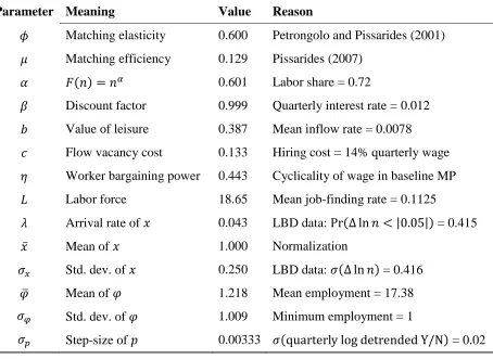
Figure 2 plots the distribution of establishment size in the calibrated model and recent data. Both axes are on a log scale to emphasize the Pareto shape of the distributions. The dots plot the empirical establishment size distribution using pooled data from the Small Business Administration on employment by firm size class for the years 1992 to 2006. The dashed line indicates the analogue implied by the calibrated model. Figure 2 reveals that the model accounts well for the empirical establishment size distribution. While this outcome is not surprising given the Pareto shocks fed through the model, it does highlight the benefit of using a flexible form for the distribution of idiosyncratic productivity in the model of sections 2 and 3.34
[FIGURE 2 HERE]
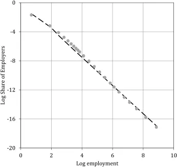
A more novel result is that the model also does a remarkable job of matching the distribution of employment growth across establishments. The dotted line in Figure 3 illustrates the empirical employment growth distribution using data for continuing es-tablishments from the Longitudinal Business Database.35 As noted above, this displays the classic features of a mass point at zero employment growth, and relatively symmet-ric tails. The dashed line overlays the employment growth distribution implied by the calibrated model, computed by time aggregation of the weekly model to annual growth rates. This bears a very close resemblance to the empirical distribution. Thus, the Pareto distribution provides a remarkably good account of the employment growth distribution, something that has not been emphasized in the literature on establishment dynamics.36
[FIGURE 3 HERE]
34The Small Business Administration (SBA) provides data on the distribution of firm size rather than establishment
size. The County Business Patterns (CBP) provides data on the latter, though the size bins are much coarser. For instance, the CBP reports the number of establishments with 20 49 workers, whereas the SBA divides this interval into six smaller bins, each with a width of 5 workers. For this reason, we prefer the SBA data. But we have reproduced the plot shown in Figure 2 with CBP data and find virtually the same pattern.
35Specifically, Figure 3 plots the cross-sectional employment growth distribution, weighting establishments equally,
as opposed to weighting by employment. The latter differ in the data (see, for example, Davis and Haltiwanger, 1992), because smaller establishments typically exhibit higher growth rate dispersion. Our simple framework does not have a mechanism to account for this feature of the data, since adjustment costs and idiosyncratic shock dispersion are invariant to firm size in the model.
36It should be noted that the model understates the literal spike at zero growth, and overstates slightly the mass just to
C. The Cyclicality of Worker Flows
It is now well-known that standard search models of the aggregate labor market cannot generate enough cyclical amplitude in unemployment, and in particular the job finding rate, to match that observed in U.S. data (Shimer 2005). A natural question is whether the generalized model analyzed here can alleviate this problem. To address this, we feed through a series of shocks to aggregate labor productivity using equation (25), and simu-late the implied dynamic response of the model using the results of section 3. Following Mortensen and Nagypal (2007), we compute the model-implied elasticities of labor mar-ket stocks and flows with respect to output per worker, and compare them with their empirical counterparts.
MODELOUTCOMES. —Panel A of Table 2 summarizes the results of this exercise. Out-comes in brackets are moments that the model is calibrated to match: the mean levels of the job-finding rate f , the unemployment inflow rate s, and the vacancy-unemployment ratio . The aim of the exercise is to draw out the implications of the model for the outcomes that the model is not calibrated to match, i.e. the cyclical elasticities of these outcomes with respect to output per worker.
[TABLE 2 HERE]
The results in Table 2.A are remarkably encouraging: On all dimensions, the model-implied elasticities lie in a neighborhood close to the cyclicality observed in the data. Specifically, the model implies an elasticity of the job finding rate of 2:55, a little below its empirical analogue of 2:65.37 In addition, the model-generated cyclical elasticity of the unemployment inflow rate of 1:64 lies only a little below the magnitude observed in the data.
COMPARISON WITHMORTENSEN ANDPISSARIDES(1994). —These results make substan-tial progress relative to the standard Mortensen and Pissarides (1994) model. To see this, panels B and C of Table 2 provide two comparison exercises.38 First, taking as given the process for idiosyncratic shocks implied by the distribution of employment growth de-rived above, we calibrate the standard model to match the mean levels of the job finding rate f and the unemployment inflow rate s, as well as the elasticity of s with respect to o