DIGITAL SELF-TUNING PID CONTROL OF PRESSURE PLANT
WITH CLOSED-LOOP OPTIMIZATION
Gediminas Liaučius, Vytautas Kaminskas, Raimundas Liutkevičius
Vytautas Magnus University, Department of Systems Analysis Vileikos St. 8, LT-3035 Kaunas, Lithuania
e-mail: [email protected], [email protected], [email protected]
Abstract. In this paper we propose a method for optimization of closed-loop parameters and continuous-time
sampling period by digital self-tuning PID control of pressure plant. The quality of pressure plant control is expe-rimentally compared between two modifications of digital self-tuning PID controllers. The results of adaptive pressure plant control show that the optimization of closed-loop parameters and sampling period provides significantly im-proved control performance.
Keywords: pressure plant, self-tuning PID controller, closed-loop parameters, sampling period, optimization.
1. Introduction
Nowadays, modern modelling, simulation, adapta-tion and intellect methods in control systems of va-rious technological processes and plants are used [1, 5, 7-9, 11]. Technological processes commonly are nuous-time plants. For the digital control of conti-nuous-time plant a sampling period of the signals is necessary to choose, which impacts the closed-loop characteristics [2].In digital PID control, the closed-loop characteristics are commonly decided by two parameters – the natural frequency of oscillation and the damping factor. The digital self-tuning PID control based on direct model identification is associated with the discrete model building and online identification of its parameters. Sampling period influences the location of the roots of model polynomials in the unit circle. On a short sampling period, the roots of model polynomials locate close to the limit of stability domain. In the process of online identification, this can cause the discrete model to become unstable [6]. All of this affects control error.
In this paper, a new method, as a solution for this problem, is proposed – the closed-loop parameters and sampling period are chosen by optimizing the control quality criterion. The experimental investigation of method effectiveness for pressure plant is performed by comparing two digital self-tuning PID controllers [10].
2. The plant
The scheme of pressure plant is demonstrated in Figure 1. The plant consists of four main components: the combined air inlet (no. 1) and outlet (no. 4) tanks, two air chambers (no. 2) and two tubes (no. 3) with balls (no. 6) in them. The air from the inlet tank flows to air channels through air chambers and leaves the equipment through the upper outlet tank. The distance to balls is measured using ultrasound distance sensors (no. 5). The fans (no. 7) are used to create pressure in the air channels in order to lift the balls in tubes. The air chambers are utilized for the purpose to stabilize oscillations of the pressure in each tube.
Figure 1. The scheme of pressure plant
The momentum of the fan, the inductance of the fan motor, air turbulence in the tube leads to complex physics governing ball's behaviour. Slightly different
weights of the balls and the location of air feeding vent additionally impact the behaviour of ball in the tubes.
The input signals of the plant are the voltage values for each fan and the output signals are the dis-tances between balls and the bottom of their tubes in centimetres.
The control objective of pressure plant is to regu-late the speed of a fan supplying the air into a tube so as to keep a ball suspended at some predetermined le-vel in the tube.
Such plants exist in air conditioning and cooling systems.
The elements of control system and technical cha-racteristics of the plant are as follows: the volume of air inlet tank is about 7000 cm3, the diameter of air feeding valve – 7 cm. The volume of each air chamber is about 1300 cm3. Each tube is 110 cm long with a diameter of 4 cm. The volume of air outlet tank is about 2900 cm3, the diameters of air outlet vents - 6.5 cm. The weights of the balls for the first and for the second tube are 3.62 g. and 3.58 g. respectively. For each air chamber, two coupled “Zalman PS80252H” fans are utilized and “Nivelco Microsonar UTP-212-4” ultrasound sensors are used for sensing the positions of the balls. The Beckhoff BK9000 PLC is used for digital control of pressure plant, i.e. reading output signals from sensors and sending input signals to the control mechanism of the fans. Controller is configured and controlled by TwinCat software.
3. Digital self-tuning PID controllers
The tubes of pressure plant are defined by discrete linear second order models, that is
, )
( )
( 1 () () 1 () () ) ( i t i t i i t i u z B y z
A (1)
, (2)
)
( () 2
2 1 ) ( 1 1 ) ( z b z b z
Bi i i
, (3)
1 )
( () 2
2 1 ) ( 1 1 ) ( z a z a z
Ai i i
where denotes the tube of the plant, , – output and input
signals with sampling period , respectively, – a white noise of the tube with a zero mean and finite variance and
2 , 1 i ) ( 0 ) ( tT yi th i ) 0 tT 0 T ) (
yti (
) ( ) (
u uti i
th i 1 ) (i t
z is the backward-shift operator.
The digital control of pressure plant is modelled by two types of digital self-tuning PID controllers: PID-A and PID-B [10]. The PID-A controller is defined as [10]
, ) ( )
( 1 () () 1 () ) ( i t i i t i e z R u z
S (4)
), 1 )( 1 ( )
( 1 1 () 1
)
(
z z
z
Si i (5)
, )
( 2() 2
1 ) ( 1 ) ( 0 1 ) ( z r z r r z
Ri i i i (6)
, (7)
) ( * ) ( ) ( i t i t i
t y y
e
where is a reference signal, - a control error and are the parameters of PID-A controller of the tube.
* ) (i t y ( 0 ) ( , i i r ) (i t e ) ( 2 ) ( 1 ) , ,ri ri
th i
In order to calculate the parameters of PID-A cont-roller the desired polynomial of closed-loop characte-ristic is needed, which for the tube is formulated as th i
nd
j d j i j i n z d z D 1 ) ( 1 ) ( , 4 , 1 )
( (8)
and is defined by converting continuous-time second order system
, (9)
0
2 2
2
i i i s
s
to its discrete analogue by Laplace transformation. The coefficients of this polynomial are then calculated by [4] , 0 ), 2 exp( , 1 ), 1 cosh( ) exp( 2 1 ), 1 cos( ) exp( 2 ) ( 4 ) ( 3 0 ) ( 2 2 0 0 2 0 0 ) ( 1 i i i i i i i i i i i i i i i i d d T d if T T if T T d (10)
where i is the natural frequency of oscillation, i is
the damping factor.
The parameters of PID-A controller are computed by [4] , ) ( 2 ) ( 2 ) ( 2 ) ( i i i i a b r
(11)
), 1
(
1 () ()
1 ) ( 1 ) ( 1 ) ( 0 i i i i i a d b
r (12)
), 1 ( () 2 ) ( 1 ) ( 2 ) ( 1 ) ( 2 ) ( 2 ) ( 2 ) (
1 i i i i i i i i a a b b r b a
r (13)
)], )( [( () 1 ) ( 2 ) ( 2 ) ( 1 ) ( 2 ) ( 1 ) ( 2 ) ( 2 i i i i i i i i b a b a b b a
r (14)
), ( () 2 ) ( 1 ) ( 2 ) ( 2 ) ( 1 ) ( 2 ) ( 2 ) ( 2 i i i i i i i i b d b d b b a
r (15)
, ] ) ( ) ( ][
[ () 2
2 2 ) ( 1 ) ( 2 ) ( 2 ) ( 1 ) ( 1 ) ( 2 ) ( 1 ) ( 2 ) ( 2 ) (
2 i i i i i i i i i i i b b a b b a b b r r r
(16)
The PID-B controller is defined as [10]
, (17)
) ( )
( 1 () () () () 1 () ) ( i t i i t i i t i y z R e u z
S
), 1 )( 1 ( )
( 1 1 () 1
)
(
z z
z
Si i (18)
. ) ( ) 1 )( 1 ( ) ( 2 ) ( 2 1 ) ( 2 ) ( 0 ) ( 0 1 ) ( 0 ) ( 2 1 ) ( 0 1 ) ( z r z r r r z r r z r z R i i i i i i i i (19)
The parameters of PID-B controller of the tube are computed by [4]
th i
), 1
(
1 ()
0 ) ( 1 ) ( ) ( 1 ) ( 1 ) ( 1 )
( i i i i i
i i r b a d
b
(20)
, ) ( 2 ) ( 2 ) ( 2 ) ( i i i i a b r
(21)
, ) ( () 2 ) ( 2 ) ( 2 ) ( 1 ) ( 2 ) ( 1 ) ( 2 ) ( 0 i i i i i i i i b a a a b b r
)], ( ) ( [ () 2 ) ( 2 ) ( 1 ) ( 2 ) ( 1 ) ( 1 ) ( 2 ) ( 2 ) ( 2 i i i i i i i i i a d b b b a b a
r (23)
], ) ( ) 1 ( )
[( () 2
1 ) ( 2 ) ( 1 2 ) ( 2 ) ( 2 ) ( 2 i i i i i i b a d b a
r (24)
. ] ) ( ) ( ][
[ () 2
2 2 ) ( 1 ) ( 2 ) ( 2 ) ( 1 ) ( 1 ) ( 2 ) ( 1 ) ( 2 ) ( 2 ) (
2 i i i i i i i i i i i b b a b b a b b r r r
(25)
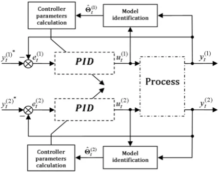
Since the model parameters of each tube are unknown, the technique of adaptive control with indirect adaptation [3, 4] is applied (Figure 2).
Figure 2. The scheme of digital self-tuning PID control
of pressure plant
The unknown model parameters of the tube are obtained by recursive least squares algorithm with forgetting factor [4]
th i , , ˆ 1 ˆ 1 , ˆ ˆ ) ( ) ( ) ( 1 ) ( ) ( 1 ) ( ) ( ) ( ) ( 1 ) ( otherwise z or e if i t i t i t i t i t i j i e i t i t i t φ C Θ Θ
Θ (26)
], ˆ , ˆ , ˆ , ˆ [ ˆ () 2 ) ( 1 ) ( 2 ) ( 1 )
(iT i i i i t a a b b
Θ (27)
], , , , [ () 2 ) ( 1 ) ( 2 ) ( 1 ) ( 1 i t i t i t i t T i
t y y u u
φ (28)
, ) ( 1 ) ( ) ( 1 ) ( i t i t T i t i
t φ C φ
(29)
, ˆ ˆ () 1 ) ( 1 ) ( ) ( i t T i t i t i
t y Θ φ
(30)
, 0 , 0 , ) ( ) ( 1 ) ( ) ( ) ( 1 ) ( 1 ) ( 1 ) ( 1 ) ( 1 ) ( 1 ) ( i t i t i t i t i t i t T i t i t i t i t i t if if C C φ φ C C
C (31)
, 1 ) ( 1 ) ( ) ( ) ( i t i i i t
(32)
where is the estimated vector of model parame-ters, – a square covariance matrix, – a data
vector, – the prediction error, – the
forget-ting factor, – auxiliary variables, – a constant that defines the admissible interval of control error and are the roots of polynomial
of the tube.
) ( ˆ i Θ ) (i ) ( ˆi ) 1 C (z ) (i φ ) (i ) ( ) ( , i i 2 , 1 , ) ( j i j th i ) (i e z ˆ Ati
In the modification of the algorithm (26), the estimates of model parameters are updated only if the value of is outside of the admissible interval
de-fined by and the model after its last estimation remains stable. ) (i t e ) (i e
4. Closed-loop optimization
The required control response or error of closed-loop by digital self-tuning PID-A or PID-B controllers can be achieved by appropriate selection of i,i,T0
parameters of the ith tube.
The control quality of the tube can be defined by criterion th i , ] ) ( ) [( 1 ) , , ( 1 2 ) ( 1 ) ( 2 ) ( * ) ( 0
N t i t i t i t i t i ii y y u u
N T
Q (33)
where N is the number of observations, 0 is a weight coefficient.
In such a case, it is reasonable to find parameters that minimize criterion (33)
* 0 * *
,
, i T
i
. (34)
) min( ) , , ( : , , 0 , , 0 * 0 * * T i i i i i i i i Q T Q T
This problem is solved using sub-component opti-mization methodology [6]
0 ) min( ) , , ( : ) min( ) , , ( : , 0 ) ( ) ( ) ( 0 , ) 1 ( 0 ) ( ) ( T i j i j i i j i j i i i j i j i Q T Q T Q T Q i i
j1,2,(35)
Each of those problems is solved as follows. Since the functions ), , , ( ) ( 0 ) ( ) ( 0 ) ( T Q T J j i j i i j
i (36)
at the stage in sub-component optimization are one-variable functions, it is reasonable to use one of the most effective direct search method – golden sec-tion method for their minimizasec-tion [6]. Search algo-rithm is related with an initial uncertainty interval
th j ], , 0 [ ] , [ () max 0 04 01 j T T
T (37)
reduction to the interval
, ],
,
[ 0()
) ( 01 ) ( 04 ) ( 04 ) ( 01 j L L L L T T T if T
T (38)
where its length is not longer than desired , and with a function (36) minimum inside.
) ( 0 j T
For this purpose, at the iteration of the search procedure two new values of sampling period are chosen th j 0 T , ) ( 618 . 0 ) ( 382 . 0 ) ( 01 ) ( 01 ) ( 04 ) ( 03 ) ( 01 ) ( 01 ) ( 04 ) ( 02 l l l l l l l l T T T T T T T T
(39)
Sampling period at the stage in sub-component optimization is then calculated by
) ( 0
j
T jth
. 2
) ( 04 ) ( 01 ) ( 0
L L j T T
T (41)
The maximum sampling period is obtained by [2]
) (
max 0
j
T
. 6 . 0
) ( ) (
max
0 j
i j
T
(42)
The functions of two variables ) , , ( ) ,
( 0( 1)
)
( j
i i i i i j
i Q T
F (43)
are also minimized using sub-component optimization method, where the golden section algorithms, analo-gous to (37) – (42), are used for the search of the para-meters i and i.
The optimization of closed-loop parameters and sampling period is performed offline.
The reference signals with representative spectral density must be applied in order to satisfy closed-loop identifiability conditions [6]. A step form signal or the signal with step changes are examples of such refe-rence signal.
5. Experimental analysis
The pressure plant has been experimentally ana-lysed using two types of digital self-tuning PID controllers – PID-A and PID-B. The same closed-loop characteristics have been used for digital control of both tubes. The initial parameters of the algorithm (26) are as follows: the main diagonal of covariance matrix ) is selected equal to 1000 while the rest
entries are equal to zero, the forgetting factor is equal to 0.99 and initial values of model parameters’ vector are set to zero. The same reference signal
for both tubes has been applied which has a step form of repeatable values of 75 and 40, and with equal to 1. The observation time of each signal is 1000 se-conds, collecting data from the plant at one-second intervals. Only the last 800 values of the signals are included in criterion calculation, thereby eliminating the impact of the initial controller training process from it. The weight coefficient
(i
C
) ( 0
ˆ i
Θ
) (i
) (i e
of criterion is set to 9 (in general, the control error of the tube is up to 90 centimetres, whereas the differences between two individual values of input signal can be up to 10 volts).
The results of criterion optimization showed that optimal closed-loop parameters and sampling period for PID-A control are *i =0.17, =0.9,
*
i
0.08,
* 0
T i1,2 , and
for PID-B control. The minima of (33) with optimal closed-loop parameters and sampling period for the first and the second tubes of PID-A control are 65.82 and 49.40 respectively, while in PID-B control - 45.36 and 36.46, i.e. the minimal values of criterion of PID-B control as compared to PID-A are less than 31% for the first tube and 26% for the second.
0.15, =
*
i
0
2. 1,
0.9, =
*
i
08 . 0
* 0
T
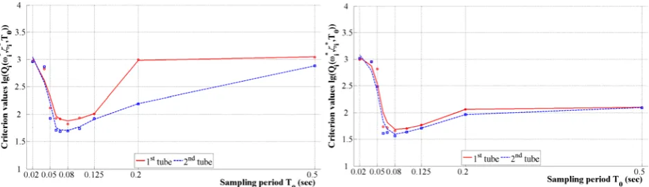
Figure 3 illustrates the dependency of control quality on sampling period with optimal closed-loop parameters Points (circles and squares) in graphs denote criterion values of each tube and curves depict the smoothed version of those values. We can see that the values of criterion of each tube little vary when sampling period is between 0.06 and 0.125, but significantly increase if the sampling period is chosen outside of this range.
T ,
*
i
i*, i
0 T
Figure 3. The influence of sampling period T0 on criterion values with optimal closed-loop parameters
0.9 = 0.17,
= *
*
i
i
for PID-A (left-hand graph) and i* =0.15,i* =0.9 for PID-B (right-hand graph)
The dependency of control quality on closed-loop parameters i, i,i1,2. with a fixed sampling
pe-riod is demonstrated in Figures 4 and 5. Notice that the closed-loop selected with natural frequency
Figure 4. Criterion values of PID-A control of each tube on various closed-loop parameters i, i with sampling
period T0 0.1
Figure 5. Criterion values of PID-B control of each tube on various closed-loop parameters i, i with sampling
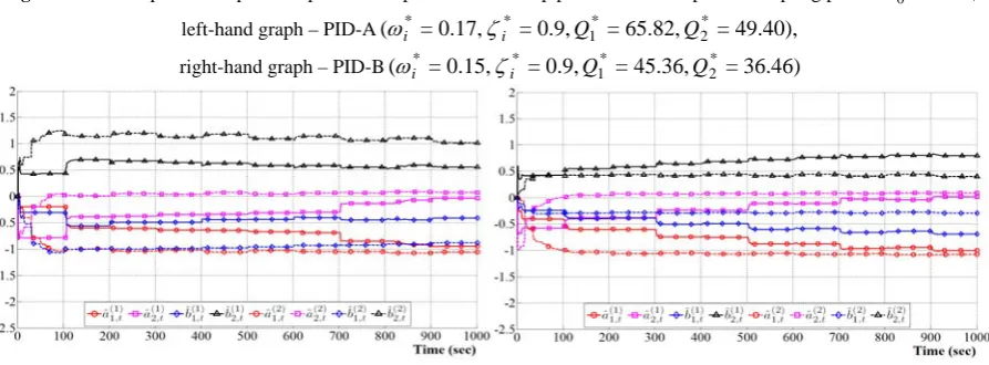
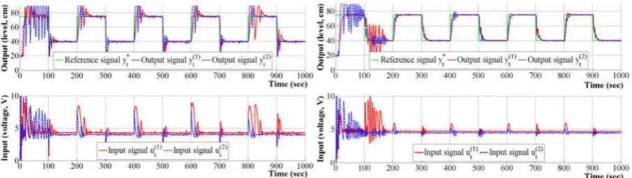
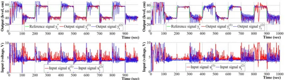
period T0 0.1 The process of adaptive pressure plant digital
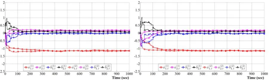
cont-rol with optimal parameters of closed-loop and opti-mal sampling period is depicted in Figure 6 and model
parameters of online identification of each pressure plant tube are depicted in Figure 7.
Figure 6. Control process of pressure plant with optimal closed-loop parameters and optimal sampling period
left-hand graph – PID-A right-hand graph – PID-B
, 08 . 0
* 0 T
49.40), = 65.82, = 0.9, = 0.17, =
(i* i* Q1* Q*2
36.46) = 45.36, = 0.9, = 0.15, =
( *2
* 1 *
* Q Q
i
i
Figure 7. Online identification of pressure plant with optimal closed-loop parameters and optimal sampling period,
Figure 8. Control process of pressure plant with optimal closed-loop parameters and sampling period left-hand graph – PID-A
right-hand graph – PID-B
, 1 . 0
0 T
54.55), = 85.16, = 0.9, = 0.17, =
( 1 2
*
* Q Q
i
i
43.31) = 50.09, = 0.9, = 0.15, =
(i* i* Q1 Q2
Figure 9. Control process of pressure plant with optimal closed-loop parameters and sampling period
left-hand graph – PID-A right-hand graph – PID-B
, 05 . 0
0 T
83.51), = 130.52, = 0.9, = 0.17, =
( 1 2
* *
Q Q
i
i
304.84) = 650.16, = 0.9, = 0.15, =
(i* i* Q1 Q2
Figure 10. Online identification of pressure plant with optimal closed-loop parameters and sampling period T0 0.05,
left-hand graph – PID-A, right-hand graph – PID-B Figure 8 shows the control process of the plant
with optimal closed-loop parameters and sampling pe-riod shifted to Notice that a small increase of sampling period slightly increases the values of criterion. The control results of the plant with optimal closed-loop parameters, but with decreased sampling period almost twice ( ) from its optimal va-lue (Figure 9) show that the choice of too small samp-ling period substantially decreases the quality of
adap-tive control. Model parameters of online identification of each pressure plant tube are illustrated in Figure 10. .
1 . 0
0 T
0 T
0 T 0.05
Åström and Wittenmark recommends to select na-tural frequency i and sampling period so that
inequality
0 T
6 . 0 1
.
0 iT0 would be valid [2].
Figu-re 11 illustrates that the selection of sampling period is unable to improve the performance of adaptive control with selected closed-loop parameter
0 T
i
recommendation causes to choose a relatively big i
with a relatively small or vice versa. Figure 12 presents the control process of the plant with a big value of
0 T
i
and a small , when its model parameters of online identification of each pressure plant tube are presented in Figure 13. The control process of pressure plant with a small value of
0 T
i
and
a big is depicted in Figure 14. In both cases, the quality of adaptive control is heavily decreased as compared to the control quality of the plant with optimal closed-loop parameters ( ) and optimal
sampling period , which are obtained by (33) and (34).
0 T
* *
, i
i
* 0 T
Figure 11. The influence of sampling period T0 on criterion values with closed-loop parameters
0.9 = 1.0, =
i i
for PID-A (left-hand graph) and PID-B (right-hand graph)
Figure 12. Control process of pressure plant with closed-loop parameters i =1.0,i =0.9 and sampling period T0 0.1,
left-hand graph – PID-A(Q1 =1673.02,Q2 =3001.57), right-hand graph – PID-B(Q1=1794.74,Q2 =2951.48)
Figure 13. Online identification of pressure plant with closed-loop parameters i =1.0,i =0.9 and sampling period
left-hand graph – PID-A control, right-hand graph – PID-B control ,
Figure 14. Control process of pressure plant with closed-loop parameters i =0.2,i =1.0 and sampling period T0 1.0, left-hand graph – PID-A(Q1=200.28,Q2 =180.40), right-hand graph – PID-B(Q1=231.37,Q2 =161.02) 6. Conclusions
The optimization method of closed-loop parame-ters and sampling period for continuous-time plant digital control has been proposed. The experimental results showed that the quality of digital self-tuning PID control of the pressure plant substantially depends on the right choice of closed-loop parameters and con-tinuous-time sampling period. Additionally, we have shown that control quality of the plant is significantly improved by optimizing those parameters. The opti-mal values of natural frequency and sampling period for digital control of pressure plant substantially differ from those that are chosen using conventional metho-dology.
References
[1] A.G. Ak, G. Cansever, A. Delibasi. Robot Trajectory
Tracking with Adaptive RBFNN-Based Fuzzy Sliding Mode Control. Information Technology and Control,
2011, Vol.40, 151-156.
[2] K.J. Åström, B. Wittenmark. Computer-Controlled
Systems: Theory and Design. New Jersey: Prentice Hall, Third Edition, 1997.
[3] K.J. Åström, B. Wittenmark. Adaptive control.
Rea-ding, Massachusetts: Addison-Wesley, 1989.
[4] V. Bobál, J. Böhm, J. Fessl, J. Macháček. Digital
Self-tuning Controllers. London: Springer-Verlag, 2005.
[5] V. Galvanauskas. Adaptive pH Control System for
Fed-Batch Biochemical Processes. Information Tech-nology and Control, 2009, Vol.38, 225-231.
[6] V. Kaminskas. Dynamic System Identification via
Discrete-time Observation: Part 1. Statistical Method Foundation. Estimation in Linear Systems, Vilnius: Mokslas Publishers, 1982 (in Russian), 245.
[7] V. Kaminskas, R. Liutkevičius. Adaptive Fuzzy
Control of Pressure and Level. Information Technolo-gy and Control, 2009, Vol.38, 232-236.
[8] R. Koerfer, R. Simutis. Advanced Process Control
for Fluidized Bed Agglomeration. Information Tech-nology and Control, 2008, Vol.37, 285-293.
[9] D. Levišauskas, V. Galvanauskas, V. Čipinytė, S.
Grigiškis. Optimization of Feed-Rate in Fed-Batch
Culture Enterobacter Aerogenes 17 E13 for Maximi-zation of Biomass Productivity. Information Technolo-gy and Control, 2009, Vol. 38, 102-107.
[10] R. Ortega, R. Kelly. PID self-tuners. Some
theore-tical and practheore-tical aspects. IEEE Trans. Ind. Electron., Vol. 31, 1984, 332-338.
[11] G. Valiulis, R. Simutis. Particle Growth Modelling