Ant Colony Optimization Approach Based Genetic Algorithms for Multiobjective Optimal Power Flow Problem under Fuzziness

(1)

Ant Colony Optimization Approach Based Genetic

Algorithms for Multiobjective Optimal Power

Flow Problem under Fuzziness

Abd Allah A. Galal1,2, Abd Allah A. Mousa1,3, Bekheet N. Al-Matrafi1

1_{Department of Mathematics and Statistics, Faculty of Sciences, Taif University, Taif, KSA} 2_{Physics and Engineering Mathematics Department, Faculty of Engineering, Tanta University, Tanta, Egypt} 3_{Department of Basic Engineering Science, Faculty of Engineering, Menoufia University, Shibin Al Kawm, Egypt}

Email: [email protected], [email protected]

Received January 2, 2013; revised February 2, 2013; accepted February 9, 2013

Li-cense, which permits unrestricted use, distribution, and reproduction in any medium, provided the original work is properly cited.

ABSTRACT

In this paper, a new optimization system based genetic algorithm is presented. Our approach integrates the merits of both ant colony optimization and genetic algorithm and it has two characteristic features. Firstly, since there is instabilities in the global market, implications of global financial crisis and the rapid fluctuations of prices, a fuzzy representation of the optimal power flow problem has been defined, where the input data involve many parameters whose possible values may be assigned by the expert. Secondly, by enhancing ant colony optimization through genetic algorithm, a strong robustness and more effectively algorithm was created. Also, stable Pareto set of solutions has been detected, where in a practical sense only Pareto optimal solutions that are stable are of interest since there are always uncertain- ties associated with efficiency data. The results on the standard IEEE systems demonstrate the capabilities of the proposed approach to generate true and well-distributed Pareto optimal nondominated solutions of the multiobjective OPF.

Keywords: Ant Colony; Genetic Algorithm; Fuzzy Numbers; Optimal Power Flow

1. Introduction

The OPF optimizes a power system operating objective function (such as the operating cost of thermal resources) while satisfying a set of system operating constraints, including constraints dictated by the electric network. OPF has been widely used in power system operation and planning. In its most general formulation, the OPF is a non-linear, non-convex, large-scale, static optimization problem with both continuous and discrete control variables. Even in the absence of non-convex unit operating cost functions, unit prohibited operating zones, and discrete control variables, the OPF problem is nonconvex due to the existence of the nonlinear (AC) power flow equality constraints. The presence of discrete control variables, such as switchable shunt devices, transformer tap positions, and phase shifters, further complicates the problem solution [1-3]. Since there is instabilities in the global market, implications of global financial crisis and the rapid fluctuations of prices, for this reasons a fuzzy representation of the multiobjective optimal power flow has been defined, where the input data involve many

parameters whose possible values may be assigned by the experts. In practice, it is natural to consider that the possible values of these parameters as fuzzy numerical data which can be represented by means of fuzzy subsets of the real line known as fuzzy numbers. Mathematical programming approaches, such as nonlinear programming, quadratic programming and linear programming, have been used for the solution of the OPF problem [4,5]. Unfortunately, the OPF problem is a highly nonlinear and a multimodal optimization problem. Therefore, con- ventional optimization methods that makes use of deriva- tives and gradients, in general, not able to locate or iden- tify the global optimum. On the other hand, many mathematical assumptions such as analytic and differen- tial objective functions have to be given to simplify the problem. Furthermore, this approach does not give any information regarding the trade-offs involved.

(2)

algorithms over the past few years have shown that these methods can be efficiently used to eliminate most of dif- ficulties of classical methods. Since they are population- based techniques, multiple Pareto-optimal solutions can, in principle, be found in one single run.

Recently, to meet the ever increasing demands in the design problems, a new evolutionary algorithm called ant colony optimization algorithm have all been used suc- cessfully to mimic the corresponding natural, or physical, or social phenomena [10-12]. Ant colony optimization (ACO) is a metaheuristic inspired by the shortest path searching behavior of various ant species. Since the initial work of Dorigo, Maniezzo, and Colorni on the first ACO algorithm, the ant system [13], several researchers have designed ACO algorithms to deal with multiobjective problems. The set of solutions achieved by a multiobjective evolutionary algorithm is required to satisfy both convergence and diversity criteria [14].

This paper intends to present a new hybrid algorithm for solving optimal power flow under fuzziness. The proposed approach integrates the merits of both ACO and GA and it has two characteristic features. Firstly, a fuzzy representation of the optimal power flow problem has been defined. Secondly, by enhancing ACO through GA, a strong robustness and more effectively algorithm was created. Several optimization runs of the proposed approach will be carry out on the standard IEEE systems to verify the validity of the proposed approach.

This paper is organized as follows. In Section 2, MOO is described. Section 3, provides a multiobjective formulation of EELD Problem. In Section 5, the proposed algorithm is presented. Implementation of the proposed approach is presented in Section 6. Results are given in Section 6. Finally, Sections 7 and 8 gives a brief discus-sion and concludiscus-sion about this study.

2. Defination of Multiobjective Optimization

A multiobjective Optimization Problem (MOP) can be defined as determining a vector of design variables within a feasible region to minimize a vector of objective functions that usually conflict with each other. Such a problem takes the form:

   





 

1 2

Minimize , , ,

subject to 0,

m





f X f X f X

g X 

Λ

where X is vector of decision variables; fi

 

X is the

ith objective function; and g X

 

is constraint vector. A decision vector X is said to dominate a decision vector Y (also written as X φY ) iff:

 

i i

f X  f Y

 

i i

for all i



1, 2, ,Λm



and f X  f Y for at least one i



1, 2,Λ,m



All decision vectors that are not dominated by any

other decision vector are called nondominated or Pareto- optimal. These are solutions for which no objective can be improved without detracting from at least one other objective.

3. Multiobjective Formulation of EELD

Problem

The economic emission load dispatch involves the si- multaneous optimization of fuel cost and emission objectives which are conflicting ones. The deterministic problem is formulated as described below.

Fuel Cost Objective. The classical economic dispatch problem of finding the optimal combination of power generation, which minimizes the total fuel cost while satisfying the total required demand can be mathemati- cally stated as follows:

 





1

2

1

$ hr

n

t i Gi

i n

i i Gi i Gi

i

f C C P

a b P c P



  

  



where

C: total fuel cost



$ hr



; Ci: is fuel cost of generator i;

, ,

i i i

a b c P

: fuel cost coefficients of generator i;

Gi

n: number of generator.

: power generated (p.u) by generator i;

Emission Objective. The emission function can be presented as the sum of all types of emission considered, such as NOx, SO2, thermal emission, etc., with suitable

pricing or weighting on each pollutant emitted. In the present study, only one type of emission NOx is taken

into account without loss of generality. The amount of NOx emission is given as a function of generator output,

that is, the sum of a quadratic and exponential function:

 









2 NO

2 2

1

10 exp ton hr

x

n

i i Gi i Gi i i Gi i

f E

P P P

    





 

 





_    _

where,     _i, , , ,_i _i _i _i: coefficients of the ith generator’s NOx emission characteristic.

Constraints: The optimization problem is bounded by the following constraints:

Power balance constraint. The total power generated must supply the total load demand and the transmission losses.

loss 1

0

n

Gi D i

P P P



  



where PD: total load demand (p.u.), and : transmis-

sion losses (p.u.). loss

(3)







loss

1 1

n n

ij i j i j ij i j i j i i

P A P P Q Q B Q P P

 







_    Q



_

where

, ,

i Gi Di i Gi Di

P P P Q Q Q









cos , sin

ij ij

ij i j ij i j

i j i j

R R

A B

V V   V V 

   

n: number of buses;

ij

R V

: series resistance connecting buses i and j;

i: voltage magnitude at bus i; i

 : voltage angle at bus i;

i

Q

P: real power injection at bus i;

i: reactive power injection at bus i.

 Maximum and Minimum Limits of Power Gen- eration. The power generated PGi by each generator

is constrained between its minimum and maximum limits, i.e.,

min max

, , , 1, ,

Gi Gi Gi

i i i

P P P

Q Q Q

V V V i

 

   Λn

where Gimin: minimum power generated, and : maximum power generated.

P PGimax

 Security Constraints. A mathematical formulation of the security constrained EELD problem would require a very large number of constraints to be considered. However, for typical systems the large proportion of lines has a rather small possibility of becoming over- loaded. The EELD problem should consider only the small proportion of lines in violation, or near violation of their respective security limits which are identified as the critical lines. We consider only the critical lines that are binding in the optimal solution. The detection of the critical lines is assumed done by the experiences of the decision maker DM. An improvement in the security can be obtained by minimizing the following objective function.

 



 

max



1

k

Gi j G j

j

S f P T P T



 



where, T_j

 

P_G

P

is the real power flow is the maximum limit of the real power flow of the jth line and k is the number of monitored lines. The line flow of the jth line is expressed in terms of the control variables _Gs, by utilizing the generalized generation distribution factors (GGDF) [1] and is given below.

max j T

 





1 n J G ji

i

T P D P





_Gi

where, ji is the generalized GGDF for line j, due to

generator i. D

For secure operation, the transmission line loading

is restricted by its upper limit as

l

S

max, 1, , SλSλ λ Λnλ

where nλis the number of transmission line.

 Multiobjective Formulation of EELD Problem. The multiobjective EELD optimization problem is therefore formulated as:

 





 









2 1 1 2 NO 2 2 1 Loss 1 max Line min max min max min max

Min $ hr

Min

10 exp ton hr

. . 0,

, 1, , , , 1, ,

, 1, , ,

x

n

t i i Gi i Gi i

n

i i Gi i Gi i i Gi i

n

Gi D i

Gi Gi Gi Gi Gi Gi i i i

f x C a b P c P

f E

P P P

s t P P P

S S n

P P P i n

Q Q Q i n

V V V i

                  _    _             



λ λ λ Λ

Λ Λ

1, ,n

 Λ

4. The Proposed Approach

This section presents a new hybrid algorithm for solving optimal power flow under fuzziness. The proposed approach integrates the merits of both ACO and GA and by enhancing ACO through GA, a strong robustness and more effectively algorithm was created. The main steps of the MACO are summarized as follows.

Step 1: Construct Q Colonies. In a multiobjective optimization problem, multiobjective functions



1, 2, , Q



F f f Λ f need to be optimized simultaneously, there does not necessarily existence a solution that is best with respect to all objectives because of incommensura- bility and confliction among objectives. For this step, the number of colonies is set to Q with its own pheromone structure, where Q F is the number of objectives to optimize.

Step 2: Initialization. First, pheromones trails are initialized to a given value ₀q,



1, 2, , where ₀

q

  ΛQ



q_is

the pheromone information in the current iteration and Pareto set are initialized to an empty set.

Implementing the multipheromone ant colony optimization for a certain problem requires a representation of n variables for each ant, with each variable i has a set of options (nodes) with their values ij which we generate

(a fully connected graph

ni l



n n, i



, and their associated pheromone oncentrations

 

ij (see Figure 1); where

1, 2, ,

i Λn, and j1, 2,Λ,ni. The process starts by

generating m ants’ position (solutions) from the population which is generated randomly, thus each ant k,



1, 2, ,



[image:3.595.310.535.87.346.2]

(4)

[image:4.595.58.288.75.222.2]

Figure 1. Ant representation.

to the associated pheromone with this value. This process continues for each objective. Consequently, path of each ant was consisted of nodes with a value for each node.

n lij

Step 3: Evaluation. The MACO parameterized by the number of ant colonies and the number of associated pheromone structures. All the colonies have the same number of ants. Each colony tries to optimize an objective considering the pheromone information associated for each colony, where each colony is determined knowing only the relevant part of a solution. This methodology enforces both colonies to search in different regions of the nondominated front.

Q



, 1, 2, ,

k k ΛQ





Step 4: Trail Update and Reward Solutions. When up- dating pheromone trails, one has to decide on which of the constructed solutions laying pheromone. The quantity of pheromone laying on a component represents the past experience of the colony with respect to choosing this component. Then, at each cycle every ant constructs a solution, and pheromone trails are updated. Once all ants have constructed their solutions, pheromone trails are updated as usually in Equation (2): first, pheromone trails are reduced by a constant factor to simulate evaporation to prevent premature convergence; then, some pheromone is laid on components of the best solution. Accordingly, pheromone concentration

associated with each possible route (variable value) is changed in a way to reinforce good solutions, as in Equation (2) and the change in pheromone concentration

 







q , 1, 2, , , 1, 2, , & 1, 2, ,

ij

p t q ΛQ i Λn j Λni

q ij



 is expressed in equation

, for Min

, for Max , if is chpsen by ant 0, otherwise

q q

q

ij q q ij

C f f

C f f l K

  

 _ 

 

A possibility is to reward every nondominated solution of the current cycle as follows

  

1

 

1



1, 2, , &

q q

ib t ib t ib

b B B ni

where q

 

ib t

 the revised concentration of pheromone is associated with option bni at iteration , t ibq



t1



is the concentration of pheromone at the previous iteration



t1



; ibq is change in pheromone concentration that

can be determined according to Equation (6); and B is the size of reward solutions

Step 5: Solution Construction. Once the pheromone is updated after an iteration, the next iteration starts by changing the ants’ paths (i.e. associated variable values) in a manner that respects pheromone concentration and also some heuristic preference. For each ant and for each dimension construct a new candidate group to replace the old one. As such, an ant will change the value for each variable according to the transition probability. The transition probability is done for each colony

k

 



q , 1, 2, ,



ij

p t q ΛQ as expressed in the following equation.

 

, ,

0, otherwise

q ij

q q

ij ij

h ni

t

j h ni

p t t



 



 _ _

 _ _



 _ _

 



where q

 

ij

p t is Probability that option is chosen by ant k for variable i at iteration t.

ij

l

Step 6: Nondominated Solutions. The set of nondominated solutions is stored in an archive. During the optimization search, this set, which represents the Pareto front, is updated. At each iteration, the current solutions obtained are compared to those stored in the Pareto archive; the dominated ones are removed and the nondominated ones are added to the set.

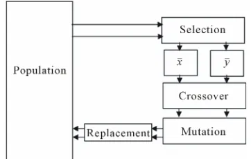
Step 7: Steady State Genetic Algorithm. Steady state genetic algorithm was implemented in such way that, two offspring are produced in each generation. Parents are selected to produce offspring and then a decision is made as to which individuals in the population to select for deletion to make room for the new offspring (Figure 2). A replacement/deletion strategy defines which member of the population will be replaced by the new offspring. Steady state genetic algorithms overlapping systems, since parents and offspring compete for survival.

,

q

   

     

[image:4.595.332.513.600.715.2]

(5)

1) Selections: Selection determines which individuals of the population will have all or some of their genetic material passed on to the next generation of individuals. The mechanism for selecting the parents is based on a tournament selection. Tournament selection operates by choosing some individuals randomly from a population and selecting the best from this group to survive into the next generation. For example, pairs of parents



x y,



are randomly chosen from the initial population. Their fitness values are compared and a copy of the better performing individual becomes part of the mating pool. The tournament will be performed repeatedly until the mating pool is filled. That way, the worst performing patent in the population will never be selected for inclusion in the mating pool. Tournaments are held between pairs of individuals are the most common. In this way all parents necessary for a reproduction operator are selected.

2) Recombination through Crossover and Mutation: After selection has been carried out, then the mechanisms of crossover and mutation are applied to produce an offspring, the following subsection outlines these genetic operators.

Crossover: Once the parents are created, the crossover step is carried out by replacing the current value with a new one which produced stochastically with a probability proportional to the crossover probability. Suppose the crossover probability set by the system is c. Generating

a random number

p

 

0,1

r r

, the crossover operation could be carried out only if pc. Suppose x and y are

two parents and  is a random number (i.e.  

 

0,1 ). The result of crossover operation x and y can be obtained by the following linear combination of x and

y:









1 1

x x y

y x

 

y

 

   

   

Mutation: Once the, the crossover is performed, the mutation step is carried out by replacing the current value with a new one which produced stochastically with a probability proportional to the mutation probability m.

Generating a random number

p

 

0,1 r

r p

, the mutation operation is implemented only if m. Suppose x j

 

will be transformed into x

 

j after mutation as follows:

 



   



,

1, 2, ,

x j L j U j L j

j n



   

 Λ

where  is a random number (i.e.  

 

0,1 ). Here L and U are the lower and upper bounds respectively.

3) Replacement/deletion strategy: A widely used combination is to replace the worst individual only if the new individual is better. In the paper, this strategy will be suggested that the individual will be deleted if it was dominated by the new offspring as in Algorithm 1.

Algorithm 1. The strategy of deletion.

1. INPUT: POP x,

2. if  x POP xφx, then

3. POP POP

4. else if  x POP xφx, then

5. POP@POPΥ   x x

6. end if

7. Output: POP

5. Implementation of the Proposed

Approach

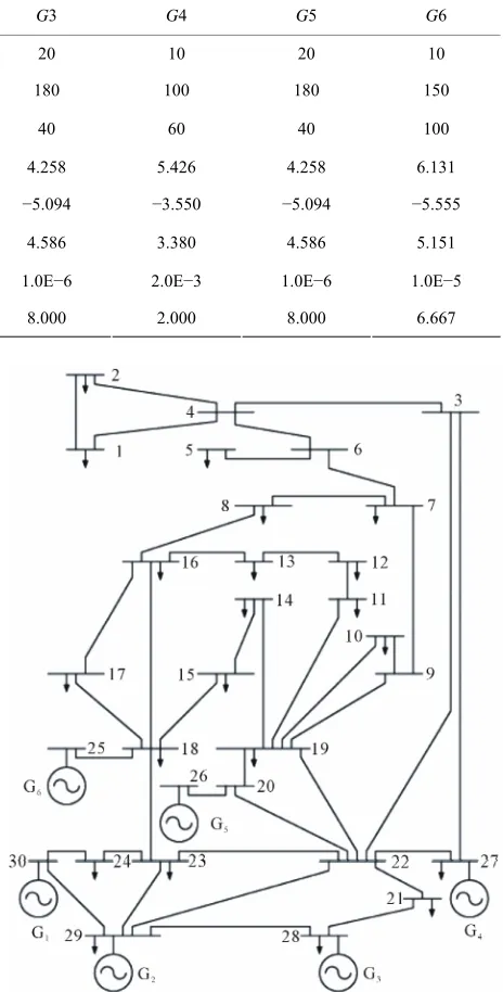
The described methodology has been described for M- objective function, but it is applied to the standard IEEE 30-bus 6-generator test system with two objectives. The single-line diagram of this system is shown in Figure 3 and the detailed data are given in [1,2]. The values of fuel cost and emission coefficients are given in Table 1. For comparison purposes with the reported results, the system is considered as losses and the security constraint is re-leased. The techniques used in this study were developed and implemented on 1.7-MHz PC using MATLAB envi-ronment. Table 2 lists the parameter setting used in the algorithm for all runs.

Naturally, these data (cost and emission) involve many controlled parameters whose possible values are vague and uncertain. Consequently each numerical value in the domain can be assigned a specific “grade of membership” where 0 represents the smallest possible grade of membership, and 1 is the largest possible grade of membership. Thus fuzzy parameters can be represented by its membership grade ranging between 0 and 1.

The fuzzy numbers shown in Figure 4 have been obtained from interviewing DMs or from observing the instabilities in the global market and rate of prices fluctuations. The idea is to transform a problem with these fuzzy parameters to a crisp version using -cut level. This membership function can be rewritten as follows:

 

1,

20 _{19, 0.95}

20

21 , 1.05

0, 0.95 or 1.05

ij

jk ij ij

ij

ij ij ij

ij ij

a a a

a a

a

a a a

a

a a a



 



 _ _{ }

  

   

 

 

 a

So, every fuzzy parameter ijcan be represented using

the membership function. By using a

[image:5.595.327.516.586.679.2]

(6)

[image:6.595.306.538.105.562.2]

Table 1. Generator cost and emission coefficients.

G1 G2 G3 G4 G5 G6

a 10 10 20 10 20 10

b 200 150 180 100 180 150 Cost

c 100 120 40 60 40 100

 4.091 2.543 4.258 5.426 4.258 6.131

 −5.554 −6.047 −5.094 −3.550 −5.094 −5.555

 6.490 4.638 4.586 3.380 4.586 5.151

 2.0E−4 5.0E−4 1.0E−6 2.0E−3 1.0E−6 1.0E−5 Emission

 2.857 3.333 8.000 2.000 8.000 6.667

Table 2. Parameters for the proposed approach.

Parameters

Number of objective function (Q) 2

Number of colonies 2

m 100

 0.5

 1

 0

C 100

0

 10

c

p 0.85

m

p 0.02

Figure 4. Consequently, each -cut level can be represented by the two end points of the alpha level.

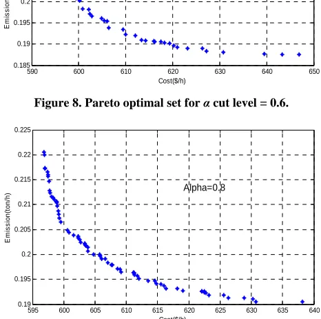
6. Results and Discussion

[image:6.595.311.536.604.713.2]

Here, the problem is how to determine the optimal power flow for considering the minimum cost and the minimum emission objectives simultaneously. In order to efficiently and effectively obtain the solution, the search for the optimal solution is carried out in two steps. Firstly, a set of nondominated solutions is obtained by exploring the optimal Pareto frontier using different  cut level. To study the influence of fuzzy parameters on the obtained Pareto optimal solutions, all the range of the parameter fluctuation were scanned, two bounds of Alpha value have been considered  0,  1, and also we take some values between these bounds  0.2,   0.4, 0.6,  0.8. Based on the definition of Pareto stability, the Pareto frontier may be reduced to a manageable size (i.e., Stable Pareto optimal solutions). MM- ACO is employed to deal with this problem. Graphical

Figure 3. Single line diagram of IEEE 30-bus 6-generator test system.

(Parameter values)

a

1.05aij ij

a

ij

a

Level  

L ij

a U

ij

a



 

(7)

presentations of the experimental results on the six in- stances problem and are presented in Figures 5-10. It is obvious from Figures 5-10 that the results maintain the diversity and convergence for all  cut level.

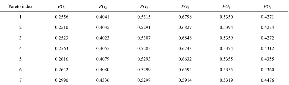
Further we need to determine stable Pareto set solution, which is a Pareto optimal for all runs (different  cut level), there was 7 Pareto solution was detected as a stable Pareto solution. Table 3 lists the set of the stable set of optimal solution. On the basis of the application, we can conclude that the proposed method can provide a sound optimal power flow by simultaneously considering multiobjective problem.

In this section, a comparative study has been carried out to assess the proposed approach concerning Pareto solutions, DM preference, and computational time. On the one hand, evolutionary techniques suffer from the large-size of the Pareto set. Therefore the proposed approach has been used to reduce the Pareto front by detecting the stable Pareto solutions under uncertainty which enable the proposed approach to help the DM to take correct decision by visualizing the Pareto front, also it maintains the di-

570 580 590 600 610 620 630 640

0.17 0.18 0.19 0.2 0.21 0.22

Cost($/h)

E

m

is

s

ion (

ton/

h)

Alpha=0

[image:7.595.309.539.87.192.2]

Figure 5. Pareto optimal set for α cut level = 0.

580 590 600 610 620 630 640

0.18 0.19 0.2 0.21 0.22 0.23

Cost($/h)

E

m

issi

o

n

(

to

n

/h

)

[image:7.595.306.539.134.365.2]

Alpha=0.2

Figure 6. Pareto optimal set for αcut level = 0.2.

580 590 600 610 620 630 640

0.18 0.19 0.2 0.21 0.22 0.23

Alpha=0.4

Cost($lh)

E

m

is

s

ion (

T

on/

[image:7.595.56.289.341.719.2]

h)

590 600 610 620 630 640 650

0.185 0.19 0.195 0.2 0.205 0.21 0.215

Alpha=0.6

Cost($/h)

E

m

is

s

ion (

ton/

h)

Figure 8. Pareto optimal set for α cut level = 0.6.

595 600 605 610 615 620 625 630 635 640 0.19

0.195 0.2 0.205 0.21 0.215 0.22 0.225

Alpha=0.8

Cost($/h)

E

m

is

s

ion

(t

on

/h

[image:7.595.59.286.352.451.2]

)

595 600 605 610 615 620 625 630 635 640 645 0.19

0.195 0.2 0.205 0.21 0.215 0.22 0.225

Alpha=1.0

Cost($lh)

E

m

is

s

ion(

ton/

h)

Figure 10. Pareto optimal set for αcut level = 1.0. versity of the solutions and good distribution over the nondominated front and take the DM preference into consideration by choosing appreciate  cut level. On the other hand, classical techniques aim to give a single point at each iterations of problem solving. On the contrary, the proposed approach generates a set of solutions at each iteration according to DM preference. Finally, the feasi- bility of using the proposed approach to handle multiobjective optimization problems has been empirically ap- proved.

7. Conclusions

[image:7.595.310.538.393.528.2] [image:7.595.58.287.615.715.2]

(8)

[image:8.595.57.540.101.243.2]

Table 3. The stable optimal pareto solutions by MM-ACO.

Pareto index PG1 PG2 PG3 PG4 PG5 PG6

1 0.2556 0.4041 0.5315 0.6798 0.5350 0.4271

2 0.2510 0.4035 0.5291 0.6827 0.5394 0.4274

3 0.2523 0.4023 0.5307 0.6848 0.5359 0.4272

4 0.2563 0.4055 0.5285 0.6743 0.5374 0.4312

5 0.2616 0.4079 0.5293 0.6632 0.5355 0.4355

6 0.2642 0.4080 0.5299 0.6594 0.5355 0.4360

7 0.2990 0.4336 0.5298 0.5914 0.5319 0.4476

[3] M. S. Osman, M. A. Abo-Sinna and A. A. Mousa, “Epsi-lon-Dominance Based Multiobjective Genetic Algorithm for Economic Emission Load Dispatch Optimization Problem,” Electric Power Systems Research, Vol. 79, No. 11, 2009, pp. 1561-1567.doi:10.1016/j.epsr.2009.06.003

optimization solution algorithms, in this paper; we proposed a new optimization system MM-ACO for solving multiobjective optimization with an application in optimal power flow considering two objectives (cost and emission). Our approach has two characteristic features. Firstly, a set of nondominated solutions is obtained by exploring the optimal Pareto frontier using different -cut level and subsequently, based on the definition of Pareto stability, the Pareto frontier may be reduced to a manageable size (i.e., Stable Pareto optimal solutions). The main features of the proposed algorithm could be summarized as follows:

[4] Y. J. Feng, L. Yu and G. L. Zhang, “Ant Colony Pattern Search Algorithms for Unconstrained and Bound Con-strained Optimization,” Applied Mathematics and Com-putation, Vol. 191, No. 1, 2007, pp. 42-56.

doi:10.1016/j.amc.2006.09.142

[5] B. Baran and M. Schaerer, “A Multiobjective Ant Colony System for Vehicle Routing Problem with Time Win-dows,” Proceedings of 21st IASTED International Con-ference on Applied Informatics, Innsbruck, 10-13

Febru-ary 2003, pp. 97-102. 1) The proposed approach is capable of determining

the stable Pareto optimal solution with two objectives, with no limitation in handing higher dimensional problems.

[6] M. Azzam and A. A. Mousa, “Using Genetic Algorithm and Topsis Technique for Multiobjective Reactive Power Compensation,” Electric Power Systems Research, Vol.

80, No. 6, 2010, pp. 675-681.

doi:10.1016/j.epsr.2009.10.033

2) The size of the Pareto optimal set has been effectively reduced to a manageable size with no further in-

formation from DM. [7] A. A. Mousa, R. M. Rizk-Allah and W. F. Abd El-Wahed, “A Hybrid Ant Colony Optimization Approach Based Local Search Scheme for Multiobjective Design Optimi-zations,” Electric Power Systems Research, Vol. 81, No.

4, 2011, pp. 1014-1023.doi:10.1016/j.epsr.2010.12.005

3) Empirically, we demonstrate that our algorithm yields consistently better results.

The performance improvement of ACO algorithm still remain in the experimental stage for lack of solid theo- retical support; thus, for future work, we intend to test the algorithm on more complex real-world applications. Also, conduct research on the parallel mechanism of the ant colony optimization algorithms so that it improves the efficiency of the algorithm used in the intelligent systems.

[8] A. A. Mousa and K. A. Kotb, “Hybrid Multiobjective Evolutionary Algorithm Based Technique for Economic Emission Load Dispatch Optimization Problem,” Scien-tific Research and Essays, Vol. 7, No. 25, 2012, pp. 2242-

2250.doi:10.5897/SRE11.197

[9] E. Zitzler and L. Thiele, “Multiobjective Evolutionary Algorithms: A Comparative Case Study and the Strength Pareto Approach,” IEEE Transactions on Evolutionary Computation, Vol. 3, No. 4, 1999, pp. 257-271.

REFERENCES

_[10] _{S. Goss, S. Aron, J. L. Deneubourg and J. M. Pasteels,} “The Self-Organizing Exploratory Pattern of the Argen-tine Ant,” Journal of Insect Behavior, Vol. 3, No. 2, 1990,

pp. 159-168. doi:10.1007/BF01417909 [1] R. Yokoyama, S. H. Bae, T. Morita and H. Sasaki,

“Mul-tiobjective Generation Dispatch Based on Probability Security Criteria,” IEEE Transactions on Power Systems,

Vol. 3, No. 1, 1988, pp. 317-324.doi:10.1109/59.43217 [11] B. Baran and M. Schaerer, “A Multiobjective Ant Colony System for Vehicle Routing Problem with Time Win- dows,” Proceedings of 21st IASTED International Con- ference on Applied Informatics, Innsbruck, 10-13 Febru-ary 2003, pp. 97-102.

[2] A. Farag, S. Al-Baiyat and T. C. Cheng, “Economic Load Dispatch Multiobjective Optimization Procedures Using Linear Programming Techniques,” IEEE Transactions on Power Systems, Vol. 10, No. 2, 1995, pp. 731-738.

(9)

“Ant Colony Optimization for the Two-Dimensional Loading Vehicle Routing Problem,” Computers & Op-erations Research, Vol. 36, No. 3, 2009, pp. 655-673.

doi:10.1016/j.cor.2007.10.021

[13] M. Dorigo and T. Stützle, “Ant Colony Optimization,” MIT Press, Cambridge, 2004.doi:10.1007/b99492 [14] M. S. Osman, M. A. Abo-Sinna and A. A. Mousa, “IT-

CEMOP: An Iterative Co-Evolutionary Algorithm for Multiobjective Optimization Problem with Nonlinear

Constraints,” Journal of Applied Mathematics & Compu-tation, Vol. 183, No. 1, 2006, pp. 373-389.

doi:10.1016/j.amc.2006.05.095

[15] B. S. Kermanshahi, Y. Wu, K. Yasuda and R. Yokoyama, “Environmental Marginal Cost Evaluation by Non-Infe- riority Surface,” IEEE Transaction on Power Systems,