Analysis and Design of Robust Quasilogarithmic Quantizer for the Purpose of Traffic Optimization

Analysis and Design of Robust

Quasilogarithmic Quantizer for the

Purpose of Traffic Optimization

ITC 4/47

Journal of Information Technology and Control

Vol. 47 / No. 4 / 2018 pp. 615-622

DOI 10.5755/j01.itc.47.4.20668

Analysis and Design of Robust Quasilogarithmic Quantizer for the Purpose of Traffic Optimization

Received 2018/04/25 Accepted after revision 2018/11/08

http://dx.doi.org/10.5755/j01.itc.47.4.20668

Corresponding author: [email protected]

Danijela Aleksić

Telekom Srbija, Voždova 11-13, 18000 Niš, Serbia, e-mail: [email protected]

Zoran Perić

University of Niš, Faculty of Electronic Engineering, Department of Telecommunications, Aleksandra Medvedeva 14, 18000 Niš, Serbia, e-mail: [email protected]

This paper proposes a simple manner to determine the support region of the quasilogarithmic robust quan-tizer. We assume Laplacian probability density function which is widely accepted as a typical model for audio and speech signals in many applications in science and engineering. Theoretically, the adaptability and robust-ness are seemingly conflicting properties, while the numerical results point out at the fact that the proposed approach to the observed support region threshold determination provides good results in a wide dynamic range from the standpoint of the signal to quantization noise ratio (SQNR). Additionally, we propose an itera-tive method for support region determination, which stops when further improvement in mean-squared error (MSE) becomes negligible. The suggested model is useful for compression schemes that involve trade-offs be-tween quantizer design and implementation complexity.

KEYWORDS: support region threshold, traffic optimization, robustness.

1. Introduction

PSTN (Public Switched Telephone Network) has been initially developed for circuit-switched traf-fic, providing a guaranteed connection between the source and the destination. Moreover, acceptable de-lay threshold is controlled through strict bandwidth allocation with each voice stream. The IP network, as originally designed data network, is additionally

crit-Information Technology and Control 2018/4/47 616

ical in most applications since the receiving end can request retransmission of the packet in question. It is well known that in a real-time constrained and latency sensitive application, such as VoIP, highly stringent delay requirements are imposed. Accord-ingly, the retransmission is not feasible since this would introduce a considerable delay prohibiting a proper two-way conversation. Thus, lost and delayed packets must be compensated for at the receiving end. Although a great number of quantizers have been developed to provide an additional QoE (quality of experience) management, especially for the VoIP ap-plications, where packet loss concealment algorithm is used [9], there is still the need to continue with re-search in this field.

Nowadays we are facing with the smart city [19] as a technology for a population, vehicles and other urban factors all of which are fused into a whole. It is obvi-ous that the data traffic generated by variobvi-ous services and application grows rapidly, which is becoming a major challenge in network architecture. 5G will bring new interactive and immersive experiences to customers, who will continue to expect new services such as augmented reality-based applications, built on high-speed and low-latency communication, with imperceptible resulting delay, jitter or interruptions [6, 4]. With more facilities being constantly added for an increased QoE (quality of experience), modern ap-plications rely heavily on the cloud for a support [3]. Beyond that, the increasing demands of user appli-cations have surged drastically and pulled up the explosive data traffic, at the same time requiring an efficient network structure to handle the data traffic all along. As the solution, offloading requires the help of some alternative networks to complement [15, 14]. Thus, transmission networks are becoming increas-ingly heterogeneous [12]. Such systems often require each node to sustain a certain throughput demand. It is essential to determine a proper transmission rate in order to guarantee the system performance that can meet the application requirement and compen-sate for the network imperfections. Such a tuning in a heterogeneous network is difficult due to the lack of modeling techniques, which can handle with the net-work traffic changes. Numerous models of quantizers have been proposed aiming at the highest possible quality of the quantized speech signals along with the highest possible compression.

In the latest years, the Internet of Things (IoT) [22] is a model including ordinary entities with the abili-ty to communicate with the corresponding devices using the Internet. There are a lot of research papers focusing on the complexities around the IoT [2] and Fog Computing, which extends the cloud closer to the things while processing the data generated by the devices. In general case, a Fog node can be any device with network connectivity, computing and storage capability, which can communicate with a variety of devices, offering a more efficient and quicker access. In addition, a further insight in the importance of the sociological aspect emphasizes the need to collect, analyze, as well as to understand the relevant back-ground of sociological processes. Non-verbal sounds such as laughing, crying, whispering, screaming, sneaking and sighing, which do not have to be accom-panied by words, can provide additional information about the individual’s attitude to a certain sociolog-ical interaction. There are many research papers which consider different communication challenges focusing on perceptual and bodily aspects of life in the modern world [13].

It is hard to predict what direction coding will take in the future. Instead of making coding obsolete, the in-terest in coding remains high nowadays.

Especially considering modern Man-Machine com-munication, we are trying to find easy and comfort-able quantization method for interaction based on speech communication. Although effective integra-tion of speech into man-machine communicaintegra-tion depends on the nature of the user interaction and application, it is preferable to minimize the influence of non-verbal behavior and the difficulties appearing in emotional or sociological background during voice communication.

The paper is structured as follows. Section 2 provides a descriptive and detailed simple solution to the prob-lem of determining the support region of the quasi-logarithmic quantizer, designed for the Laplacian source and an arbitrary variance. Section 3 is devoted at providing the numerical results and the topic. Fi-nally, related conclusions, which are summarizing the contribution achieved in the paper, are presented in Section 4.

2. Support Region of the

Quasilogarithmic Quantizer

Designed for the Laplacian PDF and

an Arbitrary Variance

The term quasi-static signal refers to a signal that chang-es so slowly over a long time so that it acquirchang-es charac-teristics more like static signals than dynamic signals [11]. The network environment requires very flexible coders that are able to adjust in real time to continu-ously changing network conditions, and particularly to varying transmission rate. In a multirate system where narrowband and wideband speech are supported, G.711 and G.722 codecs are used simultaneously.

The selection of the compression of signals and quan-tization method is a compromise between the high-est possible perceived quality of signals for the given number of bits or, conversely, minimizing the number of bits required to encode a signal at a given quality. The various compression techniques offer different levels of complexity, compressed signal quality and the amount of compressed data. It is well known that G.711 [8, 10] is a coding standard for narrowband speech and that it works on the principle of compand-ing. The codec uses A/µ-law companding technique to encode and decode speech.

Quasilogarithmic quantizer represents a logarithmic quantizer defined with the µ compression law. It is well known that, according to the G.711 coding standard, compression factor is equal to 255 [11]. Additionally, in this paper we assume various compression factors for which we analyze the performance of the proposed en-coding/decoding algorithm, coupled with G.711. In what follows, we assume that the signal at the input of the quantizer originates from a Laplacian source.

For a quasilogarithmic quantizer Q_μN_{designed for a} variance σp2, where μ is the compression factor and N is the number of quantization levels, compression is performed using the µ-law compressor functioncμ(x): [−_xσp

max,xσmaxp ] → [−xσmaxp ,xσmaxp ][11, 7]:

input of the quantizer originates from a Laplacian source. For a quasilogarithmic quantizer QμN

designed for a variance σp2, where μ is the

compression factor and N is the number of quantization levels, compression is performed using the µ-law compressor function cμ(x): [−xmaxp ,xmaxp

] → [−_xp

max,xmaxp ][11, 7]:

 

_

_

ln1 sgn

 

,

1

ln max _xmax x

x

μ μ

x x c

p p

    

  

 

  _

 (1)

for _{x x}p

max

 , wherein the _xp

max stands for the μ-law

companding quantizer’s support region threshold. For a given quantizer model wherein [xmaxp ,xmaxp ]

defines the μ-law companding quantizer’s support region, the expression for the total distortion is given by [1]:

 

_

  

  

 

 1 max 2 1

2 2 max 2 2

   

  



p p p

N _C xp xp

Q D

    

    

p p

p

x



2_exp 2 max ₍₂₎

where C = ln2_(μ+1)/(3N2_{) is a constant.}

An analysis given in [11] uncovers several insights on the relationship between granular, overload and total distortion. Additionaly, in [1], a general framework is provided for interpreting the impact of both granular and overload distortion to the number of quantization levels and the support region width.

Indeed, an N-level quantizer will be said to be globally optimal if it minimizes the expected distortion. An approach that includes estimation and optimization for a quantizer’s support region and the number of quantization levels, has proved as quite useful for designing scalar quantizers with known distributions, that were sufficiently well behaved to ensure the existence of minimal distortion [17,16]. In fact, one heuristic solution for the support region of the optimal and asymptotically optimal fixed-rate scalar quantizers has already been shown in [17]. In addition, paper [16] deals with the upper bound of this support region. A lot of quasilogarithmic quantizers were shown to be applicable to solve for the minimum distortion. In [18, 20] some solutions to the two-stage quantization model based on quasi-logarithmic quantizers are given. The prior work [21] that included backward adaptation technique, has offered a complex but improved solution to the quasilogarithmic quantizer model, preferable for the smaller compression factor values. The source coding in [5] adopts frame-by-frame processing

quantizers, while taking into consideration the unequal support regions, selected according to the lower distortion criteria.

An intention of this paper is to generalize support region estimation by giving an expression for the maximal signal amplitude and its numerical computation. Furthermore, our objective is to extend the analysis of support region _xp

max

determination to the cases where the compression factor μ has an arbitrary value. If we assume that the value of the parameter μ is large enough (for instance μ = 255 as defined by G.711 standard), we obtain the following approximate formula for total distortion _DL

 

_Q N

 :

   

N  N

L_{Q DQ}

D _{ 255}

    

    

    

  

 

p p

p p

p

p _x

x C

 

 

 2 max 2 ₁ 2_exp 2 max

. (3)

In accordance with the minimal distortion criteria, achieved by setting the first derivate of the so obtained distortion _DL

 

_QN

 to zero with respect to p

xmax:





1 _exp 2 ₀

3 1

ln max,L

2

2 p

     

     

p

x

N  

  _{, (4)}

the support region threshold _x p,L

max

 _{is derived as:}





_  

  

 

  



1 ln

3 ln

2 2

2 L

,

maxp N

x p

. (5)

According to minimal distortion criteria for the total distortion given by _D

 

_QN

 (3):



2



0

exp 2 2 2

max 2

maxp _C _{  x} p _

Cx 



 . (6)

In order to determine _xp

max the application of

iterative numerical method is required:





     

 

     

 

 

 _

p i p

i

p p

x N

x

    

 

) 1 ( max 2

2 )

( max

2 1

1 1

ln 3 ln 2

     

 

     

 



 _

p i p

p

x C

   

 ( 1)

max

2 1

1 ln

2 . (7)

(1)

for _{x x}σp max

≤ , wherein the _xσp

max stands for the μ-law companding quantizer’s support region threshold. For a given quantizer model wherein [_−xmaxσp ,_xmaxσp ]

de-fines the μ-law companding quantizer’s support re-gion, the expression for the total distortion is given by [1]:

 

_

  

  

 

 1 max 2 1

2 2 max 2 2

   

  



p p p

N _C xp xp

Q D

    

    

p p

p

x

 2_exp 2 max

, (2)

where C = ln2_(μ+1)/(3N2_{) is a constant.}

An analysis given in [11] uncovers several insights on the relationship between granular, overload and total distortion. Additionaly, in [1], a general framework is provided for interpreting the impact of both granular and overload distortion to the number of quantization levels and the support region width.

Indeed, an N-level quantizer will be said to be glob-ally optimal if it minimizes the expected distortion. An approach that includes estimation and optimiza-tion for a quantizer’s support region and the number of quantization levels, has proved as quite useful for designing scalar quantizers with known distribu-tions, that were sufficiently well behaved to ensure the existence of minimal distortion [17,16]. In fact, one heuristic solution for the support region of the optimal and asymptotically optimal fixed-rate scalar quantizers has already been shown in [17]. In addi-tion, paper [16] deals with the upper bound of this support region.

giv-Information Technology and Control 2018/4/47 618

en. The prior work [21] that included backward adap-tation technique, has offered a complex but improved solution to the quasilogarithmic quantizer model, preferable for the smaller compression factor val-ues. The source coding in [5] adopts frame-by-frame processing using the combination of two three-level restricted quantizers, while taking into consideration the unequal support regions, selected according to the lower distortion criteria.

An intention of this paper is to generalize support re-gion estimation by giving an expression for the maxi-mal signal amplitude and its numerical computation. Furthermore, our objective is to extend the analysis of support region _xσp

max determination to the cases where the compression factor μ has an arbitrary value. If we assume that the value of the parameter μ is large enough (for instance μ = 255 as defined by G.711 stan-dard), we obtain the following approximate formula for total distortion _DL

( )

_Q N

µ :

  

N  N





L_{Q DQ}

D _{ 255}

                    p p p p p p _x x C    

 2 max 2 ₁ 2_exp 2 max _. (3)

In accordance with the minimal distortion criteria, achieved by setting the first derivate of the so obtained distortion _DL

( )

_Q N

µ to zero with respect to xσmaxp : In what follows, we assume that the signal at the

input of the quantizer originates from a Laplacian source. For a quasilogarithmic quantizer QμN designed for a variance σp2_{, where μ is the} compression factor and N is the number of quantization levels, compression is performed using the µ-law compressor function cμ(x): [−_xp

max,xmaxp ] → [−_xp

max,xmaxp ][11, 7]:

 

_

_

ln 1 sgn

 

, 1

ln max _xmax x

x μ μ x x c p p             _  (1)

for _{x x}p max

 , wherein the _xp

max stands for the μ-law companding quantizer’s support region threshold. For a given quantizer model wherein [xmaxp,xmaxp ] defines the μ-law companding quantizer’s support region, the expression for the total distortion is given by [1]:

 

_        

 1 max 2 1

2 2 max 2 2         p p p

N _C xp xp

Q D           p p p x 

2_exp 2 max ₍₂₎

where C = ln2_(μ+1)/(3N2_{) is a constant.}

An analysis given in [11] uncovers several insights on the relationship between granular, overload and total distortion. Additionaly, in [1], a general framework is provided for interpreting the impact of both granular and overload distortion to the number of quantization levels and the support region width.

Indeed, an N-level quantizer will be said to be globally optimal if it minimizes the expected distortion. An approach that includes estimation and optimization for a quantizer’s support region and the number of quantization levels, has proved as quite useful for designing scalar quantizers with known distributions, that were sufficiently well behaved to ensure the existence of minimal distortion [17,16]. In fact, one heuristic solution for the support region of the optimal and asymptotically optimal fixed-rate scalar quantizers has already been shown in [17]. In addition, paper [16] deals with the upper bound of this support region. A lot of quasilogarithmic quantizers were shown to be applicable to solve for the minimum distortion. In [18, 20] some solutions to the two-stage quantization model based on quasi-logarithmic quantizers are given. The prior work [21] that included backward adaptation technique, has offered a complex but improved solution to the quasilogarithmic quantizer model, preferable for the smaller compression factor values. The source coding in [5] adopts frame-by-frame processing

using the combination of two three-level restricted quantizers, while taking into consideration the unequal support regions, selected according to the lower distortion criteria.

An intention of this paper is to generalize support region estimation by giving an expression for the maximal signal amplitude and its numerical computation. Furthermore, our objective is to extend the analysis of support region _xp

max determination to the cases where the compression factor μ has an arbitrary value. If we assume that the value of the parameter μ is large enough (for instance μ = 255 as defined by G.711 standard), we obtain the following approximate formula for total distortion _DL

 

_QN

 :

   

N  N L_{Q DQ}

D _{ 255}

                    p p p p p p _x x C    

 2 max 2 ₁ 2_exp 2 max

. (3)

In accordance with the minimal distortion criteria, achieved by setting the first derivate of the so obtained distortion _DL

 

_QN

 to zero with respect to





1 _exp 2 ₀

3 1

ln max,L

2 2 p             p x

N  

  _{, (4)}

the support region threshold _x p,L

max

 _{is derived as:}





_            1 ln 3 ln 2 2 2 L ,

maxp N

x p

. (5)

According to minimal distortion criteria for the total distortion given by _D

 

_QN

 (3):



2



0

exp 2 2 2 max 2

maxp _C _{  x} p _

Cx 



 . (6)

In order to determine _xp

max the application of iterative numerical method is required:





                   _ p i p i p p x N x        ) 1 ( max 2 2 ) ( max 2 1 1 1 ln 3 ln 2                   _ p i p p x C    

 ( 1) max 2 1

1 ln

2 . (7)

(4)

the support region threshold _x p,L

max

σ _{is derived as:}





_            1 ln 3 ln 2 2 2 L ,

maxp N

x p . (5)

According to minimal distortion criteria for the total distortion given by _D

( )

_Q N

µ (3): In what follows, we assume that the signal at the

input of the quantizer originates from a Laplacian source. For a quasilogarithmic quantizer QμN

designed for a variance σp2, where μ is the

compression factor and N is the number of

quantization levels, compression is performed using the µ-law compressor function cμ(x): [−xmaxp ,xmaxp ] → [−_xp

max,xmaxp ][11, 7]:

 

_

_

ln 1 sgn

 

,

1

ln max _xmax x

x μ μ x x c p p             _  (1)

for _{x x}p

max

 , wherein the _xp

max stands for the μ-law companding quantizer’s support region threshold. For a given quantizer model wherein [xmaxp ,xmaxp ]

defines the μ-law companding quantizer’s support

region, the expression for the total distortion is given by [1]:

 

_        

 1 max 2 1

2 2 max 2 2         p p p

N _C xp xp

Q D           p p p x 

2_exp 2 max ₍₂₎

where C = ln2_(μ+1)/(3N2_{) is a constant.}

An analysis given in [11] uncovers several insights on the relationship between granular, overload and total distortion. Additionaly, in [1], a general framework is provided for interpreting the impact of both granular and overload distortion to the number of quantization levels and the support region width.

Indeed, an N-level quantizer will be said to be globally optimal if it minimizes the expected distortion. An approach that includes estimation and optimization for a quantizer’s support region and the number of quantization levels, has proved as quite useful for designing scalar quantizers with known distributions, that were sufficiently well behaved to ensure the existence of minimal distortion [17,16]. In fact, one heuristic solution for the support region of the optimal and asymptotically optimal fixed-rate scalar quantizers has already been shown in [17]. In addition, paper [16] deals with the upper bound of this support region. A lot of quasilogarithmic quantizers were shown to be applicable to solve for the minimum distortion. In [18, 20] some solutions to the two-stage quantization model based on quasi-logarithmic quantizers are given. The prior work [21] that included backward adaptation technique, has offered a complex but improved solution to the quasilogarithmic quantizer model, preferable for the smaller compression factor values. The source coding in [5] adopts frame-by-frame processing

using the combination of two three-level restricted quantizers, while taking into consideration the unequal support regions, selected according to the lower distortion criteria.

An intention of this paper is to generalize support region estimation by giving an expression for the maximal signal amplitude and its numerical computation. Furthermore, our objective is to

extend the analysis of support region _xp

max determination to the cases where the compression factor μ has an arbitrary value. If we assume that the value of the parameter μ is large enough (for instance μ = 255 as defined by G.711 standard), we obtain the following approximate formula for total distortion _DL

 

_Q N

 :

   

N  N L_{Q DQ}

D _{ 255}

                    p p p p p p _x x C    

 2 max 2 ₁ 2_exp 2 max

. (3)

In accordance with the minimal distortion criteria, achieved by setting the first derivate of the so obtained distortion _DL

 

_QN

 to zero with respect to

p xmax:





1 _exp 2 ₀

3 1

ln max,L

2 2 p             p x

N  

  _{, (4)}

the support region threshold _x p,L max

 _{is derived as:}





_            1 ln 3 ln 2 2 2 L ,

maxp N

x p

. (5)

According to minimal distortion criteria for the total distortion given by _D

 

_QN

 (3):



2



0

exp 2 2 2 max 2

maxp _C _{  x} p _

Cx 



 . (6)

In order to determine _xp

max the application of iterative numerical method is required:





                   _ p i p i p p x N x        ) 1 ( max 2 2 ) ( max 2 1 1 1 ln 3 ln 2                   _ p i p p x C    

 ( 1)

max 2 1

1 ln

2 . (7)

(6)

In order to determine _xσp

max the application of iterative numerical method is required:





               _ p i p i p p x N x        ) 1 ( max 2 2 ) ( max 2 1 1 1 ln 3 ln 2                 _ p i p p x C    

 ( 1)

max 2 1 1 ln 2 . (7)

To accelerate the estimation of _xσp

max, we initialize the iterative method using the support region threshold obtained in (5):

Step1. Theinitialization of the algorithm: The

  _L

p

p _x

x max, 0 max   _                      C C x p x

x p pL

p        ln 1 1 ln 2 , max ) 0 ( max ) 1 ( max , (8)

where C = ln2_(μ+1)/(3N2_{) is a constant.}

Step2. The computation of new threshold value ( )2

maxp

xσ using (7) and the interruption of the iterative method if the estimated relative error defined as: To accelerate the estimation of _xp

max, we initialize the iterative method using the support region threshold obtained in (5):

Step1. The initialization of the algorithm:

  pL

p _x

x max,

0 max   _                      C C x p x x p pL p        ln 1 1 ln 2 , max ) 0 ( max ) 1 ( max , (8) where C = ln2_(μ+1)/(3N2_{) is a constant.}

Step2. The computation of new threshold value

 2 maxp

x using (7) and the interruption of the iterative method if the estimated relative error defined as:

 

%   _{ 2}   100

max 1 max 2

max  _

 p p p x x x     (9)

is less than 5·10-3_.

3. The Numerical Results

In this section, our objective is to ascertain and summarize the performances for quasilogarithmic quantizer for an arbitrary variance in a wide variance range.

Here, by identifying xp _k_p

max , according to (5)

and (8), one can come to the conclusion that _xp max can be presented by using multiplying coefficient k:

,

max k p

xp _{  (10)}













  2 , max 2 2 2 1 max 2 2

1 _ln 3 _,for

ln 1 2

3 _.

ln 1

1 ln ,for

2 ₁ 1_ln 3

ln 1 p p L N _x N k x N              _ _      _{ }           _{ }   _{  }      _{ }  _  (11)

In order to account for the deployment of quasilogarithmic quantizer and arbitrary variance

σp2 in a wide dynamic range of input variance σq2, we assume that the design for the quasilogarithmic quantizer for an arbitrary variance σq2 is based on the design of the same quantizer for the σp2 along with the scaling with the coefficient ρ_:

p q 



 / (12)

 





          

 2 1

3 1 ln 2 2 2 2 2 2     

 k k

N Q

D N q

2

_exp

2

_.

q

k





























(13)

For a given quasilogarithmic quantizer's model, the minimum distortion criterion is employed to assure the maximum of SQNR:

 

_      

 q_N

Q D _ 2 10 log 10 SQNR

 

_                   

 10log₁₀ C a2₂ 2a 1 exp 2a



 ,(14)

where ak/.

Figures 1-3 show the SQNR characteristics of the suggested quantizer for various compression factors.

Figure 1

SQNR dependence on the scaling coefficient ρ for μ=255 and R=3-8 [bit/sample]

3 4 5 6 7 8

0 5 10 15 20 25 30 35 40 45            SQNR [dB ] R[bit/sample] Figure 2

SQNR dependence on the scaling coefficient ρ for μ=10 and R=3-8 [bit/sample]

3 4 5 6 7 8

0 5 10 15 20 25 30 35 40 45            SQ NR [dB ] R[bit/sample] Figure 3 (9)

is less than 5·10-3_.

3. The Numerical Results

In this section, our objective is to ascertain and sum-marize the performances for quasilogarithmic quan-tizer for an arbitrary variance in a wide variance range. Here, by identifying xσp ₌k_σp

max , according to (5) and (8), one can come to the conclusion that _xσp

max can be presented by using multiplying coefficient k:

To accelerate the estimation of _xp

max, we initialize

the iterative method using the support region threshold obtained in (5):

Step1. The initialization of the algorithm:

  _pL

p _x

x max,

0 max   _                      C C x p x x p pL p        ln 1 1 ln 2 , max ) 0 ( max ) 1 ( max , (8) where C = ln2_(μ+1)/(3N2_{) is a constant.}

Step2. The computation of new threshold value

 2 maxp

x using (7) and the interruption of the iterative method if the estimated relative error defined as:

 

%   _{ 2}   100

max 1 max 2

max  _

 p p p x x x     (9)

is less than 5·10-3_.

3. The Numerical Results

In this section, our objective is to ascertain and summarize the performances for quasilogarithmic quantizer for an arbitrary variance in a wide variance range.

Here, by identifying xmaxp kp, according to (5)

and (8), one can come to the conclusion that _xp max

can be presented by using multiplying coefficient k: ,

max k p

xp _{  (10)}













  2 , max 2 2 2 1 max 2 2

1 _ln 3 _,for

ln 1 2

3 _.

ln 1

1 ln ,for

2 ₁ 1_ln 3

ln 1 p p L N _x N k x N              _ _      _{ }           _{ }   _{  }      _{ }  _  (11)

In order to account for the deployment of quasilogarithmic quantizer and arbitrary variance

σp2 _{in a wide dynamic range of input variance σq}2_,

we assume that the design for the quasilogarithmic quantizer for an arbitrary variance σq2 _{is based on}

the design of the same quantizer for the σp2 _along

with the scaling with the coefficient ρ_: p

q 



 / (12)

 





          

 2 1

3 1 ln 2 2 2 2 2 2     

 _N k k

Q

D N q

2

_exp

2

_.

q

k





























(13)

For a given quasilogarithmic quantizer's model, the minimum distortion criterion is employed to assure the maximum of SQNR:

 

_      

 q_N

Q D _ 2 10 log 10 SQNR

 

_                   

 10log₁₀ C a2₂ 2a 1 exp 2a



 ,(14)

where ak/.

Figures 1-3 show the SQNR characteristics of the suggested quantizer for various compression factors.

Figure 1

SQNR dependence on the scaling coefficient ρ for μ=255 andR=3-8 [bit/sample]

3 4 5 6 7 8

0 5 10 15 20 25 30 35 40 45            SQNR [dB ] R[bit/sample] Figure 2

SQNR dependence on the scaling coefficient ρ for μ=10 andR=3-8 [bit/sample]

3 4 5 6 7 8

619

Information Technology and Control 2018/4/47

To accelerate the estimation of xmax, we initialize

the iterative method using the support region threshold obtained in (5):

Step1. The initialization of the algorithm:

  _pL

p _x

x max,

0 max   _                      C C x p x x p pL p        ln 1 1 ln 2 , max ) 0 ( max ) 1 ( max , (8) where C = ln2_(μ+1)/(3N2_{) is a constant.}

Step2. The computation of new threshold value

 2 maxp

x using (7) and the interruption of the iterative method if the estimated relative error defined as:

 

%   _{ 2}   100

max 1 max 2

max  _

 p p p x x x     (9)

is less than 5·10-3_.

3. The Numerical Results

In this section, our objective is to ascertain and summarize the performances for quasilogarithmic quantizer for an arbitrary variance in a wide variance range.

Here, by identifying xmaxp kp, according to (5) and (8), one can come to the conclusion that _xp

max

can be presented by using multiplying coefficient k: ,

max k p

xp _{  (10)}













  2 , max 2 2 2 1 max 2 2

1 _ln 3 _,for ln 1

2

3 _.

ln 1

1 ln ,for

2 ₁ 1_ln 3 ln 1 p p L N _x N k x N              _ _      _{ }           _{ }   _{  }    _{ }  _  (11)

In order to account for the deployment of quasilogarithmic quantizer and arbitrary variance σp2 in a wide dynamic range of input variance σq2, we assume that the design for the quasilogarithmic quantizer for an arbitrary variance σq2 is based on the design of the same quantizer for the σp2 along with the scaling with the coefficient ρ_:

p q  

 / (12)

 





        

 2 1

3 1 ln 2 2 2 2     

 _N k k

Q

D N q

2

_exp

2

_.

q

k





























(13)

For a given quasilogarithmic quantizer's model, the minimum distortion criterion is employed to assure the maximum of SQNR:

 

_      

 q_N

Q D _ 2 10 log 10 SQNR

 

_                   

 10log₁₀ C a2₂ 2a 1 exp 2a



 ,(14)

where ak/.

Figures 1-3 show the SQNR characteristics of the suggested quantizer for various compression factors.

Figure 1

SQNR dependence on the scaling coefficient ρ for μ=255 andR=3-8 [bit/sample]

3 4 5 6 7 8

0 5 10 15 20 25 30 35 40 45            SQNR [dB ] R[bit/sample] Figure 2

SQNR dependence on the scaling coefficient ρ for μ=10 andR=3-8 [bit/sample]

3 4 5 6 7 8

0 5 10 15 20 25 30 35 40 45            SQ NR [dB ] R[bit/sample] Figure 3 (11)

In order to account for the deployment of quasiloga-rithmic quantizer and arbitrary variance σp2 in a wide dynamic range of input variance σq2, we assume that the design for the quasilogarithmic quantizer for an arbitrary variance σq2 is based on the design of the same quantizer for the σp2 along with the scaling with the coefficient ρ:

To accelerate the estimation of _xp

max, we initialize the iterative method using the support region threshold obtained in (5):

Step1. The initialization of the algorithm:

  pL

p _x

x max,

0 max   _                      C C x p x x p pL p        ln 1 1 ln 2 , max ) 0 ( max ) 1 ( max , (8) where C = ln2_(μ+1)/(3N2_{) is a constant.}

Step2. The computation of new threshold value

 2 maxp

x using (7) and the interruption of the iterative method if the estimated relative error defined as:

 

%   _{ 2}   100 max

1 max 2

max  _

 p p p x x x     (9)

is less than 5·10-3_.

3. The Numerical Results

In this section, our objective is to ascertain and summarize the performances for quasilogarithmic quantizer for an arbitrary variance in a wide variance range.

Here, by identifying xmaxp kp, according to (5)

and (8), one can come to the conclusion that _xp

max can be presented by using multiplying coefficient k:

,

max k p

xp _{  (10)}













  2 , max 2 2 2 1 max 2 2

1 _ln 3 _,for ln 1

2

3 _.

ln 1

1 ln ,for 2 ₁ 1_ln 3

ln 1 p p L N _x N k x N              _ _      _{ }           _{ }   _{  }      _{ }  _  (11)

In order to account for the deployment of quasilogarithmic quantizer and arbitrary variance σp2 in a wide dynamic range of input variance σq2,

we assume that the design for the quasilogarithmic quantizer for an arbitrary variance σq2 is based on

the design of the same quantizer for the σp2 along

with the scaling with the coefficient ρ_:

p q  

 / (12)

 





          

 2 1

3 1 ln 2 2 2 2 2 2     

 _N k k

Q

D N q

2

_exp

2

_.

q

k





























(13)

For a given quasilogarithmic quantizer's model, the minimum distortion criterion is employed to assure the maximum of SQNR:

 

_      

 q_N

Q D  2 10 log 10 SQNR

 

_                   

 10log10 C a2_{2 }2a 1 exp 2a

 ,(14)

where ak/.

Figures 1-3 show the SQNR characteristics of the suggested quantizer for various compression factors.

Figure 1

SQNR dependence on the scaling coefficient ρ for μ=255 and R=3-8 [bit/sample]

3 4 5 6 7 8

0 5 10 15 20 25 30 35 40 45            SQNR [dB ] R[bit/sample] Figure 2

SQNR dependence on the scaling coefficient ρ for μ=10 and R=3-8 [bit/sample]

3 4 5 6 7 8

0 5 10 15 20 25 30 35 40 45            SQ NR [dB ] R[bit/sample] Figure 3 (12)

 





          

 2 1

3 1 ln 2 2 2 2 2 2     

 _N k k

Q

D N q

2

_exp

2

_.

q

k





























(13)

For a given quasilogarithmic quantizer’s model, the minimum distortion criterion is employed to assure the maximum of SQNR:

To accelerate the estimation of _xp

max, we initialize the iterative method using the support region threshold obtained in (5):

Step1. The initialization of the algorithm:

  _pL

p _x

x max,

0 max   _                      C C x p x x p pL p        ln 1 1 ln 2 , max ) 0 ( max ) 1 ( max , (8) where C = ln2_(μ+1)/(3N2_{) is a constant.} Step2. The computation of new threshold value

 2 maxp

x using (7) and the interruption of the iterative method if the estimated relative error defined as:

 

%   _{ 2}   100

max 1 max 2

max  _

 p p p x x x     (9)

is less than 5·10-3_.

3. The Numerical Results

In this section, our objective is to ascertain and summarize the performances for quasilogarithmic quantizer for an arbitrary variance in a wide variance range.

Here, by identifying xmaxp kp, according to (5)

and (8), one can come to the conclusion that _xp max can be presented by using multiplying coefficient k:

,

max k p

xp _{  (10)}













  2 , max 2 2 2 1 max 2 2

1 _ln 3 _,for ln 1

2

3 _.

ln 1

1 ln ,for 2 ₁ 1_ln 3

ln 1 p p L N _x N k x N              _{ } _     _{ }           _{ }   _{  }      _{ }  _  (11)

In order to account for the deployment of quasilogarithmic quantizer and arbitrary variance

σp2 in a wide dynamic range of input variance σq2,

we assume that the design for the quasilogarithmic quantizer for an arbitrary variance σq2 is based on

the design of the same quantizer for the σp2 along

with the scaling with the coefficient ρ_:

p q 



 / (12)

 





          

 2 1

3 1 ln 2 2 2 2 2 2     

 _N k k

Q

D N q

2

_exp

2

_.

q

k





























(13)

For a given quasilogarithmic quantizer's model, the minimum distortion criterion is employed to assure the maximum of SQNR:

 

_      

 q_N

Q D _ 2 10 log 10 SQNR

 

_                   

 10log₁₀ C a2₂ 2a 1 exp 2a 

 ,(14)

where ak/.

Figures 1-3 show the SQNR characteristics of the suggested quantizer for various compression factors.

Figure 1

SQNR dependence on the scaling coefficient ρ for μ=255 andR=3-8 [bit/sample]

3 4 5 6 7 8

0 5 10 15 20 25 30 35 40 45            SQNR [dB ] R[bit/sample] Figure 2

SQNR dependence on the scaling coefficient ρ for μ=10 andR=3-8 [bit/sample]

3 4 5 6 7 8

0 5 10 15 20 25 30 35 40 45            SQ NR [dB ] R[bit/sample] Figure 3 (14)

where a=k/ρ.

Figures 1-3 show the SQNR characteristics of the suggested quantizer for various compression factors. It should be noted that for μ=10 and R =5 or 6, SQNR can range more than 15dB for the range ρ=0.2 to ρ=2, while for μ=100 and R=3 or 4, SQNR can range more than 10dB for ρ=0.2 to ρ=2. At higher bit rates, for ex-ample for R=8 and higher, for the range ρ=0.2 to ρ=2, SQNR higher than 20 or 30 dB can be obtained for μ=10 or μ=100, respectively. In this way, by selecting the parameter μ and R, and in accordance with the

Figure 1

SQNR dependence on the scaling coefficient ρ for μ=255 andR=3-8 [bit/sample]

Figure 2

SQNR dependence on the scaling coefficient ρ for μ=10 and

R=3-8 [bit/sample]

Figure 3

SQNR dependence on the scaling coefficient ρ for μ=100 andR=3-8 [bit/sample]

To accelerate the estimation of _xp

max, we initialize

the iterative method using the support region threshold obtained in (5):

Step1. The initialization of the algorithm:

  _pL

p _x

x_max 0  _max ,

                     C C x p x

x p pL

p









   ln 1 1 ln 2 , max ) 0 ( max ) 1 ( max , (8) where C = ln2_(μ+1)/(3N2_{) is a constant.}

Step2. The computation of new threshold value

 2 maxp

x using (7) and the interruption of the iterative method if the estimated relative error defined as:

 

%   _{ 2}   100

max 1 max 2

max  _

 p p p x x x   



(9)

is less than 5·10-3_.

3. The Numerical Results

In this section, our objective is to ascertain and summarize the performances for quasilogarithmic quantizer for an arbitrary variance in a wide variance range.

Here, by identifying xmaxp kp, according to (5)

and (8), one can come to the conclusion that _xp

max

can be presented by using multiplying coefficient k: ,

max k p

xp _



(10)













  2 , max 2 2 2 1 max 2 2

1 _ln 3 _,for ln 1

2

3 _.

ln 1

1 ln ,for 2 ₁ 1_ln 3

ln 1 p p L N _x N k x N  















    _{ } _     _{ }           _{ }   _{  }      _{ }  _  (11)

In order to account for the deployment of quasilogarithmic quantizer and arbitrary variance

σp2 in a wide dynamic range of input variance σq2,

we assume that the design for the quasilogarithmic quantizer for an arbitrary variance σq2 is based on

the design of the same quantizer for the σp2 along

with the scaling with the coefficient ρ_:

p

q







 / (12)

 





          

 2 1

3 1 ln 2 2 2 2 2 2











 k k

N Q

D N _q

2

_exp

2

_.

q

k















_



_









(13)

For a given quasilogarithmic quantizer's model, the minimum distortion criterion is employed to assure the maximum of SQNR:

 

_      

 q_N

Q D 



2 10 log 10 SQNR

 

_                   

 10log10 C

_

a2₂

_

2a 1 exp 2a ,(14)

where ak/.

Figures 1-3 show the SQNR characteristics of the suggested quantizer for various compression factors.

Figure 1

SQNR dependence on the scaling coefficient ρ for μ=255 andR=3-8 [bit/sample]

3 4 5 6 7 8

0 5 10 15 20 25 30 35 40 45            SQNR [dB ] R[bit/sample] Figure 2

SQNR dependence on the scaling coefficient ρ for μ=10 andR=3-8 [bit/sample]

3 4 5 6 7 8

0 5 10 15 20 25 30 35 40 45            SQ NR [dB ] R[bit/sample] Figure 3

To accelerate the estimation of _xp

max, we initialize

the iterative method using the support region threshold obtained in (5):

Step1. The initialization of the algorithm:

  pL

p _x

x_max 0  _max ,

                     C C x p x

x p pL

p









   ln 1 1 ln 2 , max ) 0 ( max ) 1 ( max , (8) where C = ln2_(μ+1)/(3N2_{) is a constant.}

Step2. The computation of new threshold value

 2 maxp

x using (7) and the interruption of the iterative method if the estimated relative error defined as:

 

%   _{ 2}   100

max 1 max 2

max  _

 p p p x x x   



(9)

is less than 5·10-3_.

3. The Numerical Results

In this section, our objective is to ascertain and summarize the performances for quasilogarithmic quantizer for an arbitrary variance in a wide variance range.

Here, by identifying xp _k_p

max , according to (5)

and (8), one can come to the conclusion that _xp max

can be presented by using multiplying coefficient k: ,

max k p

xp _

_

₍₁₀₎













  2 , max 2 2 2 1 max 2 2

1 _ln 3 _,for

ln 1 2

3 _.

ln 1

1 ln ,for

2 ₁ 1_ln 3

ln 1 p p L N _x N k x N              _ _      _{ }           _{ }   _{  }      _{ }  _  (11)

In order to account for the deployment of quasilogarithmic quantizer and arbitrary variance

σp2 in a wide dynamic range of input variance σq2, we assume that the design for the quasilogarithmic quantizer for an arbitrary variance σq2 is based on the design of the same quantizer for the σp2 along with the scaling with the coefficient ρ_:

p

q







 / (12)

 





          

 2 1

3 1 ln 2 2 2 2 2 2











 k k

N Q

D N q

2

_exp

2

_.

q

k





























(13)

For a given quasilogarithmic quantizer's model, the minimum distortion criterion is employed to assure the maximum of SQNR:

 

_      

 q_N

Q D _



2 10 log 10 SQNR

 

_                   

 10log₁₀ C a2₂ 2a 1 exp 2a





,(14)

where ak/.

Figures 1-3 show the SQNR characteristics of the suggested quantizer for various compression factors.

Figure 1

SQNR dependence on the scaling coefficient ρ for μ=255 andR=3-8 [bit/sample]

3 4 5 6 7 8

0 5 10 15 20 25 30 35 40 45            SQNR [dB ] R[bit/sample] Figure 2

SQNR dependence on the scaling coefficient ρ for μ=10 andR=3-8 [bit/sample]

3 4 5 6 7 8

0 5 10 15 20 25 30 35 40 45            SQ NR [dB ] R[bit/sample] Figure 3

SQNR dependence on the scaling coefficient ρ for

μ=100 and R=3-8 [bit/sample]

3 4 5 6 7 8

0 5 10 15 20 25 30 35 40 45            SQ N R [d B] R[bit/sample]

It should be noted that for μ=10 and R =5 or 6, SQNR can range more than 15dB for the range ρ=0.2 to ρ=2, while for μ=100 and R=3 or 4, SQNR can range more than 10dB for ρ=0.2 to ρ=2. At higher bit rates, for example for R=8 and higher, for

the range ρ=0.2 to ρ=2, SQNR higher than 20 or 30

dB can be obtained for μ=10 or μ=100, respectively.

In this way, by selecting the parameter μ and R, and

in accordance with the required minimum values of SQNR and the variance range, the choice of the performances of the quasilogarithmic quantizer can be balanced, at the same time achieving additional optimization in the amount and volume of the transferred data in bits.

The proposed support region estimation method makes possible simple initialization of the suggested algorithm. Namely, the initial value

 0

maxp

x _{for the suggested iterative method is equal to}

a L x x p max , max 

 _{, which is obtained from an}

approximate closed-form formula for the support region threshold of the quasilogarithmic quantizer designed for the Laplacian source of an arbitrary variance given in [10].

Moreover, one can notice that the suggested iterative method converges very fast. For the simplicity purpose, we can assume that determining

p

xmax is accomplished after only one itteration. In

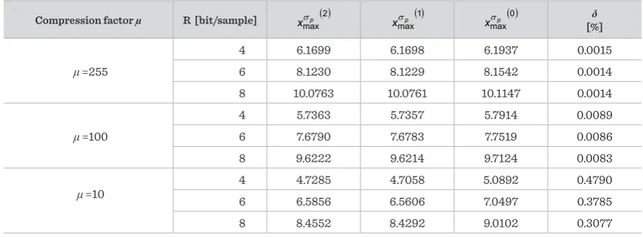
order to account for the assumption validation, the relative error of estimating the support region threshold is calculated for µ=255, µ=100, µ=10 and a different number of quantization levels N (N =16,

N = 64 and N =256), listed in Table 1. according to

(9).

Notably, the potential for the support region threshold determination with the reduced number of used bits can be highlighted. We address the problem of suitable support region threshold determination by limiting a relative error approximately to a value less than 0.5%, in the worst case.

Here, we have shown that the SQNR of the

considered quasilogarithmic quantizer is

additionally tuned using fast and accurate estimation of the support region threshold that provides minimal total distortion for the signal with an accommodated amplitude dynamic.

Table 1 Parametres for the analysis of the accuracy of the formula for the support region threshold of the quasilogarithmic quantizer

Compression factor µ R

[bit/sample] xmaxp  2  

1 maxp

x xmaxp  0 _[%] δ

4 6.1699 6.1698 6.1937 0.0015

μ=255 6 8.1230 8.1229 8.1542 0.0014

8 10.0763 10.0761 10.1147 0.0014

4 5.7363 5.7357 5.7914 0.0089

μ=100 6 7.6790 7.6783 7.7519 0.0086

8 9.6222 9.6214 9.7124 0.0083

4 4.7285 4.7058 5.0892 0.4790

μ=10 6

8 6.5856 8.4552 6.5606 8.4292 7.0497 9.0102 0.3785 0.3077

4. Conclusion

Our aim is to outline the main conclusion when the robust quantizer presents the underlying desirable solution out of the whole set of different quantizer's solutions.

To that end, we have evaluated the performance of robust quantizer without obligatory insisting on the highest SQNR values.