Performance analysis of a complex repairable system with two subsystems in series configuration with an imperfect switch

*_{Corresponding author}

E-mail address: [email protected] Received November 28, 2019

Available online at http://scik.org

J. Math. Comput. Sci. 10 (2020), No. 2, 359-383 https://doi.org/10.28919/jmcs/4399

ISSN: 1927-5307

PERFORMANCE ANALYSIS OF A COMPLEX REPAIRABLE SYSTEM WITH TWO SUBSYSTEMS IN SERIES CONFIGURATION WITH AN IMPERFECT

SWITCH

VIJAY VIR SINGH1,*_{, PRAVEEN KUMAR POONIA}2 _{AND AMEER HASSAN ADBULLAHI}3 1_{Department of Mathematics, Yusuf Maitama Sule University, Kano State, Nigeria}

2_{Department of General Requirement, Sur College of Applied Sciences, Oman}

3_{Department of Mathematics, Kano University of Science & Technology Wudil, Kano State, Nigeria} Copyright © 2020 the author(s). This is an open access article distributed under the Creative Commons Attribution License, which permits unrestricted use, distribution, and reproduction in any medium, provided the original work is properly cited.

Abstract: This paper presents the study of reliability measures of a complex system consisting of two subsystems, subsystem-1, and subsystem-2, in a series configuration with switching device. The subsystem-1 has five units that are working under 2-out-of-5: G policy and the subsystem-2 has two units that are working under 1-out-of-2: G policy. Moreover, the switching device in the system is unreliable, and as long as the switch fails, the whole system fails immediately. Failure rates of units of subsystems are constant and assumed to follow the exponential distribution. Still, their repair supports two types of distribution, namely general distribution and Gumbel-Hougaard family copula distribution. Using the supplementary variable technique, Laplace transformations, and copula approach differential equations developed. Important reliability characteristics such as availability of the system, reliability of the system, MTTF, profit analysis, and sensitivity analysis for MTTF have computed for fixed values of failure and repair rates. Particular cases corresponding to the switching device have also considered. Graphs demonstrate results, and consequently, conclusions have done.

Keywords: k-out-of-n: G system; availability; reliability; MTTF; cost analysis; Gumbel-Hougaard family-copula distribution.

1. INTRODUCTION

Complicated systems such as computers, automobiles industry, telephone networks, and various

electronic networks are becoming a prevalent feature and essential requirements of our society.

The systems are built with multiple components/ parts to perform specified tasks adequately. It is

often difficult to assure that the systems will perform particular tasks efficiently for which they

designed. Due to various causes, it is difficult to anticipate the failure of a component and

sometimes impossible to prevent the failure of the entire system. Reliability is a vital need for

proper uses and repair of any engineering system. Achieving a high or required level of reliability

and availability of the system is often an essential requisite based on system designed structure.

The importance and utility of a system depend on its successful performance, and its performance

depends on its design. The availability and reliability of an industrial system may be enhancing

using a highly reliable structural design of the system or subsystem of higher reliability. The best

way to improve system reliability is to add redundant components in the design. A constructive

and common form of redundancy is a k-out-of-n configuration. Many researchers have brought

their attention to the study of k-out-of-n: G systems and k-out-of-n: F systems. The k-out-of-n: G

system is good if and only if at least k of its n components is good, while k-out-of-n: F system fails

if and only if at least k of its n components fails. For example, an airplane with four engines can be

modeled as a 3-out-of-4: G system. Furthermore, consider a large truck with ten tires is an example

of 6-out-of-10: G system. Although the system performance may be degraded if less than ten tires

are operational, rearrangement of the tire configuration will result in adequate performance as long

as at least six tires are operational. In nuclear power plant system 2-out-of-4: G; system can

perform adequate power supply. Conclusively a k-out-of-n system plays a very crucial role in

system reliability theory to the proper operation of the system.

In the past decade, many researchers have focused on k-out-of-n-type systems mainly because

such systems are more general than pure parallel or pure series systems, and they frequently come

across in practice. There is an extensive literature available for reliability analysis of

k-out-of-n-type systems under various situation such as [10], repairable systems with different

failure modes [25], three-unit series system under warm standby [15], consecutive k-out-of-n

system using standby with multiple working vacations [19], generalized block replacement policy

with respect to a threshold number of failed components and risk costs [13], non-identical

components subject to repair priorities [1] and non-identical components considering shut-off

PERFORMANCE ANALYSIS OF A COMPLEX REPAIRABLE SYSTEM

satellites, transmission systems, or computer systems where some new equipment groups need to

add because of the requirement for better output of the system. Realizing this fact, authors like

Alka and Singh [3] analyzed reliability analysis of a complex repairable system composed of two

2-out-of-3: G subsystems connected in a parallel configuration. They analyzed the system by using

the supplementary variable technique and obtain various measures such as mean time to failure,

steady-state probability, availability, and cost analysis. Yusuf et al. [7] focus on the comparative

study of 2-out-of-3: G system for the different situations under the concept of general repair

analyzed using Kolmogorov's forward equations method. The objective of this study is to see the

effect of preventive maintenance and system design of 2-out-of-3. In addition, Yusuf et al. [8, 9]

developed an explicit expression for mean time to system failure for a 3-out-of-5 warm standby

system involving common cause failure and ensured the maximum overall MTSF of the system.

Considering one type of repair/general repair to a totally failed system may cause a massive loss

due to the non-operation of the system, and the industry/organization may drop its market

reputation. Several authors, including El-Said and EL-Sherbeny [11], Bulama et al. [12], Gupta et

al. [16, 17] and Malik et al. [20] examined the reliability characteristics under the presumption that

the failed unit can be repaired by employing only one type of repair. There are many situations in

real life where more than one repair is possible between two adjacent transition states for quick

repair of the failed system. When such type of possibility exists, the system is repaired using the

Gumbel-Hougaard family copula; it couples the two distributions, namely general distribution and

exponential distribution. Therefore, in contrast to this, authors have considered models in which

they tried to address a problem where two different repair facilities are available between adjacent

states, i.e., the initial state and totally failed state. Ram and Singh [14] have studied availability and

cost analysis of a parallel redundant complex system with two types of failure under preemptive-

resume repair discipline using the Gumbel-Hougaard family copula in repair. Singh et al. [21]

have studied cost analysis of an engineering system involving two subsystems in a series

configuration with controllers and human failure under the concept of k-out-of-n: G policy using

Gumbel-Hougaard family copula distribution. Also, in [22, 23], Singh et al. have studied the

performance analysis of the complex system in the series configuration under different failure and

repair disciplines using copula and controllers. Bona et al. [5] have discussed the reliability

allocation based integrated factor method (IFM) approach to the aerospace system. The

consequence of the study of reliability allocation method Di, Bona, Forcina, A, and Silvestri, A,

thermonuclear system. Recently Lado et al. [2] analyzed two subsystems connected in a series

configuration and operated by a human operator. In this study, they concluded that copula repair is

more reliable compared to general repair. Also, Babu et al. [4] studied a δ-shock maintenance

model for a deteriorating system with an imperfect delayed repair under partial process. In

addition, Singh and Poonia [24] studied two units parallel system with correlated lifetime under

inspection using regenerative point technique.

Authors who studied k-out-of-n systems have put attention toward the operation of units in parallel/series configuration or in a circular arrangement with catastrophic failure and preventive maintenance but did not consider transfer switch and its failure. Therefore, realizing the fact and necessity of such type of configuration, we in the present analyzing a complex system having two subsystems viz. subsystem-1 and subsystem-2 under k-out-of-n: G configuration. Both subsystems connected in series, and each linked with a switching device for the proper functioning of the system, which may be perfect or imperfect at the time of need. The subsystem-1 follows 2-out-of-5: good configuration, and subsystem-2 follows 1-out-of-2: good configuration. All the units in both the subsystems are in a parallel configuration. The system has three possible transition states: Good, partially failed and complete failed. The system may move to the failed state as per the following options:

(i) More than three units of subsystem-1 fail, but both units of subsystem-2 are in good

working condition.

(ii) Both of the units of the subsystem-2 fail.

(iii) The switching device of the subsystem-1 / subsystem-2 fails.

In addition to this, the system will be in a partially failed state in the following situations:

(i) At least one and maximum up to 3 units of subsystem-1 failed, and all the units of

subsystem-2 are good.

(ii) All units of subsystem-1 are good, and anyone unit of subsystem-2 fails.

PERFORMANCE ANALYSIS OF A COMPLEX REPAIRABLE SYSTEM

the proposed design. Section 2 to 6 covers the state description, assumptions, nomenclature of notation used for the study of a mathematical model, and transition diagram. Section 7 and 8 cover the analytical part of the paper in which some particular cases are taken for discussion and elaboration. Section 8 describes the conclusion of the study with results.

2. STATE DESCRIPTION

The description of the various possible state of the model after failing the units in both the subsystems, including transfer switch failure, is given in Table 1. The states {S0, S1, S2, S3, and S5} are operative states, and {S4, S6, S7, and S8} are inoperative states of the system.

Table 1 State Description of the model

State State description

S0 This is a perfect state, and all units of subsystem-1 and subsystem-2 are in good working condition.

S1

The indicated state represents that the system is degraded but is in operational mode after the failure of any one unit in subsystem-1, but both units of subsystem-2 are in a good operational state. The system is under repair.

S2

The indicated state represents that the system is degraded but is in operational mode after the failure of any two units in subsystem-1, but both units of subsystem-2 are in a good operational state. The system is under repair.

S3

The indicated state represents that the system is degraded but is in operational mode after the failure of any three units in subsystem-1. Still, both units of subsystem-2 are in a good operational state. The system is under repair.

S5

The indicated state represents that the system is degraded but is in operational mode after the failure of anyone unit in subsystem-2, but all the units of subsystem-1 are in a good operational state. The system is under repair.

S4 The states represent that the system is in totally failed mode after failing more than three units in the

subsystem 1. The system is under repair using the Gumbel-Hougaard family copula distribution. S6 The states represent that the system is in a complete failed state after failing both units in subsystem

2. The system is under repair using employing copula distribution. S7 It is a complete failed state due to switch failure in the subsystem-1.

3. ASSUMPTIONS

The following assumptions have been made throughout the study of the model:

1. Initially, the system is in the stateS₀, and all the units of subsystem-1 and subsystem-2 are in

good working conditions.

2. The subsystem-1 works successfully until three or more than three units are in good working

condition, i.e., 2-out-of-5:Gpolicy.

3. The subsystem-2 works successfully if one or both units are in good working condition, i.e.,

1-out-of-2:Gpolicy.

4. Both the subsystems having switching devices, which may be unreliable at the time as long

as the switch fails, the whole system fails immediately.

5. The units in both the subsystems are in parallel mode and hot standby and ready to start

within a negligible time after the failure of any unit in the subsystems.

6. Repairperson is available to full time with the system and maybe called as soon as the system

reaches to partially or totally failed state.

7. All failure rates are constant and follow the exponential distribution.

8. The complete failed system needs repair immediately. For this, copula can be employed to

restore the system.

9. No damage reported due to the repair of the system.

PERFORMANCE ANALYSIS OF A COMPLEX REPAIRABLE SYSTEM

4. NOTATIONS

t, s Time scale and Laplace transform variable

1/ 2

  The failure rate of each unit in the subsystem-1/subsystem-2.

1/ 2

s s

  The failure rate of the switching devices between the units for subsystem-

1/subsystem-2.

( ) ( )

1 x / 1 y

  The Repair rate of each unit in the subsystem-1/subsystem-2.

( )

0 z

 Repair rate of the switching device for both the subsystems.

( )

0

P t The state transition probability that the system is in stateS_i at an instanti=0.

( )

P s Laplace transformation of the state transition probabilityP t

( )

( )

P x t The probability that the system is in the stateS_i for i=1 to 8and the system is

under repair with elapsed repair time is ,x t. x is repaired variable and t is

time variable.

( )

p

E t Expected profit in the interval. [0, t)

1, 2

K K Revenue generated and service cost per unit time, respectively.

( )

0 x

 An expression of the joint probability from failed state Si to good state S0

according to Gumbel-Hougaard family copula, is given

( )



( )



 



 = _ +  _ whereu x₁

( ) ( )

( )

u x =e . Here is the parameter1   .

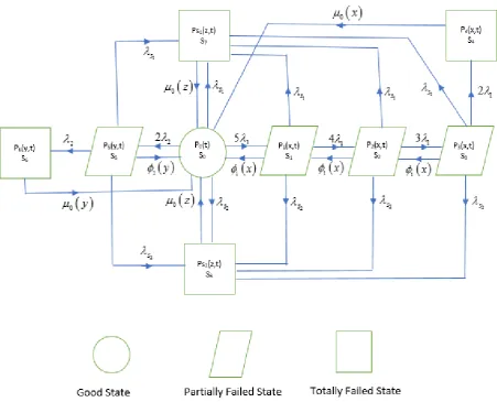
5. SYSTEM CONFIGURATION AND STATE TRANSITION DIAGRAM

System configuration is shown in Fig 1 (a) while the transition diagram in Fig 1 (b). In transition diagram, S0 is perfect state, S1, S2, S3, and S5 partial failed/degraded and S4, S6, S7, and S8 are

complete failed states. Due to failure in any unit in the subsystem-1 and in subsystem-2, the transitions approach to partially failed states S1, S2, S3, and S5, respectively. The state S4 and S6

are complete failed states due to the failure of units in both the subsystems. The states S7 and S8

Figure 1 (a) System configuration

PERFORMANCE ANALYSIS OF A COMPLEX REPAIRABLE SYSTEM

6. FORMULATION OF THE MODEL

By a probability of considerations and continuity arguments, we can obtain the following set of difference-differential equations associated with the present mathematical model:

( )

( ) ( )

( ) ( )

1 2

1 2 0 1 1 2 5

0 0

5 2 _{s s} P t x P x t dx, y P y t dy,

t      

     _{+ + + +}  _{= +}  _    





( ) ( )

( ) ( )

0 4 0 6

0 0

, ,

x P x t dx y P y t dy

 

 

+

_

_

( ) ( )

( ) ( )



0 0

0 0

, ,

s s

z P z t dz z P z t dz

 

 

+

_

_

( ) ( )

1 2

1 1 1

4 _{s s} x P x t, 0

t x    

 

 _{+ + + + +}  ₌

_{ } 

  (2)

( ) ( )

1 2

1 1 2

3 _{s s} x P x t, 0

t x    

 

 _{+ + + + +}  ₌

_{ } 

  (3)

( ) ( )

1 2

1 1 3

2 _{s s} x P x t, 0

t x    

 

 _{+ + + + +}  ₌

_{ } 

  (4)

( )





( )

exp x log x P x t, 0

t x

 

 _

 ₊  _{+  + }  ₌

_{   } 

  (5)

( ) ( )

1 2

2 s s 2 y P y t5 , 0

t y    

  

+ + + + + =

_{ } 

  (6)

( )





( )

exp y log y P y t, 0

t y    _   _{ }  + + + = _{   } 

  (7)

( )





( )

exp z log z P_s z t, 0

t z    _   _{ }  + + + = _{   } 

  (8)

( )





( )

exp z log z P_s z t, 0

t z

 

 _

 ₊  _{+  + }  ₌

_{   } 

  (9)

Boundary conditions

( )

( )

1 0, 5 1 0

( )

( )

( )

2 0, 4 1 1 0, 20 1 0

P t = P t =  P t (11)

( )

( )

( )

3 0, 3 1 2 0, 60 1 0

P t = P t =  P t (12)

( )

( )

( )

4 0, 2 1 3 0, 120 1 0

P t = P t =  P t (13)

( )

( )

5 0, 2 2 0

P t =  P t (14)

( )

( )

( )

6 0, 2 5 0, 2 2 0

P t = P t =  P t (15)

( )

( )

( )

( )

( )

( )

1 0, 1 0 1 0, 2 0, 3 0, 5 0,

s s

P t = _P t +P t +P t +P t +P t _ (16)

( )

( )

( )

( )

( )

( )

2 0, 2 0 1 0, 2 0, 3 0, 5 0,

s s

P t = _P t +P t +P t +P t +P t _ (17)

Initials conditions

( )

0 0 1

P = , and other state probabilities are zero att=0 (18)

Solution of the model

Taking Laplace transformation of equations (1) to (17) and using equation (18), we obtain

( )

( ) ( )

( ) ( )

1 2

1 2 0 1 1 2 5

0 0

5 2 s s 1 , ,

s     P s  x P x s dx  y P y s dy

 

 + + + +  = + +

 





( ) ( )

( ) ( )

0 4 0 6

0 0

, ,

x P x s dx y P y s dy

 

 

+

_

_

( ) ( )

( ) ( )



0 0

0 0

, ,

s s

z P z s dz z P z s dz

 

 

+

_

_

where

( )

( )

0

, st ,

i i

P x s e P x t dt

 −

=

_

( ) ( )

1 2

1 1 1

4 _{s s} , 0

s x P x s

x    



 _{+ + + + +}  ₌

 _ 

  (20)

( ) ( )

1 2

1 1 2

3 s s , 0

s x P x s

x    



 _{+ + + + +}  ₌

 _ 

  (21)

( ) ( )

1 2

1 1 3

2 _{s s} , 0

s x P x s

x    



 _{+ + + + +}  ₌

 _ 

PERFORMANCE ANALYSIS OF A COMPLEX REPAIRABLE SYSTEM

( )





( )

exp log , 0

s x x P x s

x

 

 _

 ₊  _{+  + }  ₌

 _{  } 

  (23)

( ) ( )

1 2

2 s s 2 5 , 0

s y P y s

y    

  

+ + + + + =

 _ 

  (24)

( )





( )

exp log , 0

s y y P y s

y    _   _{ }  + + + =  _{  } 

  (25)

( )





( )

exp log _s , 0

s z z P z s

z

 

 _

 ₊  _{+  + }  ₌

 _{  } 

  (26)

( )





( )

exp log _s , 0

s z z P z s

z

 

 _

 ₊  _{+  + }  ₌

 _{  } 

  (27)

( )

( )

1 0, 5 1 0

P s = P s (28)

( )

( )

( )

2 0, 4 1 1 0, 20 1 0

P s = P s =  P s (29)

( )

( )

( )

3 0, 3 1 2 0, 60 1 0

P s = P s =  P s (30)

( )

( )

( )

4 0, 2 1 3 0, 120 1 0

P s = P s =  P s (31)

( )

( )

5 0, 2 2 0

P s =  P s (32)

( )

( )

( )

6 0, 2 5 0, 2 2 0

P s = P s =  P s (33)

( )

( )

( )

( )

( )

( )

1 0, 1 0 1 0, 2 0, 3 0, 5 0,

s s

P s = _P s +P s +P s +P s +P s _

(

)

( )

1

2 3

1 1 1 2 0

1 5 20 60 2

s P s

    

= + + + + (34)

( )

( )

( )

( )

( )

( )

2 0, 2 0 1 0, 2 0, 3 0, 5 0,

s s

P s = _P s +P s +P s +P s +P s _

(

)

( )

2

2 3

1 1 1 2 0

1 5 20 60 2

s P s

    

= + + + + (35)

Laplace transformation of boundary conditions after repair

( )

( )

( ) ( )

1 1 0 1 2

0

0, 5 ,

P s P s  x P x s dx



= +

_

( )

( )

( )

0

3

1 0 1 2

0

5 0,

x

s s

s x x dx

P s x e P s dx

( )

(

)

( )

1 1 2

1 0 1 2

5P s S_ s 3 _s _s P 0,s

= + + + +

( )

(

)

( )

1 1 2

1 0 1 1 1

5P s S s 3 s s 4P 0,s

= + + + +

( )

₍

₎

( )

1 1 2

1

1 0

1 1

5 0,

1 4 3 _{s s}

P s P s

S_ s 

   

=

− + + + (36)

Similarly

( )

₍

₎

( )

1 1 2

2 1 2 0 1 1 20 0,

1 3 2 _{s s}

P s P s

S_ s



   

=

− + + + (37)

( )

( )

₍

₎

( )

1 1 2

3 1

3 1 2 0

1 1

60

0, 3 0,

1 3 2 _{s s}

P s P s P s

S_ s

 

   

= =

− + + + (38)

( )

( )

₍

₎

( )

1 1 2

4 1

4 1 3 0

1 1

120

0, 2 0,

1 3 2 s s

P s P s P s

S s

 

   

= =

− + + + (39)

( )

( )

5 0, 2 2 0

P s =  P s (40)

( )

( )

( )

6 0, 2 5 0, 2 2 0

P s = P s =  P s (41)

( )

(

)

( )

1 1

2 3

1 1 1 2 0

0, 1 5 20 60 2

s s

P s = +  +  +  +  P s (42)

( )

(

)

( )

2 2

2 3

1 1 1 2 0

0, 1 5 20 60 2

s s

P s = +  +  +  +  P s (43)

Now solving all the equations with the boundary conditions, one may get

( )

_{( )}

( )

_{( )}



(

)



(

)



(

)



1 1

1

1 1 1

1 4

5

4 1 4 3

s s

s s s s

S s

P s

D s _{s S s}

             − + + + =

+ + + − + + + (45)

( )

_{( )}



(

)



(

)



(

)



2

1 1

2

1 1 1

1 3

20

3 1 3 2

s s

s s s s

S s

P s

D s _{s S s}

             − + + + =

+ + + − + + + (46)

( )

_{( )}



(

)



(

)



(

)



3

1 1

3

1 1 1

1 2

60

2 1 3 2

s s

s s s s

S s

P s

D s _{s S s}

             − + + + =

PERFORMANCE ANALYSIS OF A COMPLEX REPAIRABLE SYSTEM

( )

_{( )}



( )



(

)





1 1 2

4 1 4 1 1 1 120

1 3 2 _{s s}

S s P s

D s s S s

       − =

− + + + (48)

( )

_{( )}



₍

(

₎

)



2 s s

s s

S s P s

D s s

   



  

− + + +

=

+ + + (49)

( )

_{( )}



( )



2 2 6

1

2 S s

P s

D s s

  −

= (50)

( )

(

_{( )}

)



( )



2 3

1 1 1 2 1

1 5 20 60 2

s s

S s

P s

D s s



 +  +  +  +  −

= (51)

( )

(

_{( )}

)



( )



2 3

1 1 1 2 1

1 5 20 60 2

s s

S s

P s

D s s



 +  +  +  +  −

= (52)

where

( )

1 2

4

2

1 1

1 2 2 2

1 1

5 120

5 2 2 2

1 4 1 3

s s

P T

D s s S T

Q R           = + + + + − − − − − −

(

)

(

)

2 3

1 1 1 2

1 5 20 60 2

s s T

     

− + + + + +

and

(

)

1 1 2

1 2 1 1 1 1 4 4 s s s s

P S s

s          = + + + = + + + +

(

)

1 1 2

1 2 1 1 1 1 3 3 s s s s

Q S s

s          = + + + = + + + +

(

)

1 1 2

1 2 1 1 1 1 2 2 s s s s

R S s

s          = + + + = + + + +

(

)

2 1 2

1 2 2 2 2 2 s s s s

S S s

s          = + + + = + + + +

( )

s

 _

= =

+

Sum of Laplace transformations of the state transitions, where the system is in operational mode and failed state at any time, is as follows.

( )

( )

( )

( )

( )

( )

up

( )

(

)





(

)

_

(

)

_

(

)





(

)



(

)



(

)





(

)



(

)



(

)





1 1 2

1 2 1 1 2

1 1 2

1 2 1 1 2

1 1 2

1 2 1 1 2

2 1 2

1 1

1 1 1

2

1 1

1 1 1

3

1 1

1 1 1

2 2

5 1 4

1

4 1 4 3

20 1 3

3 1 3 2

1

60 1 2

2 1 3 2

2 1

s s

s s s s

s s

s s s s

s s

s s s s

s s

S s

s S s

S s

s S s

D s _{S s}

s S s

S s s                                             − + + + + + + + − + + + − + + + + + + + − + + + = − + + + + + + + − + + + − + + + + +

(

)

                              + +     (53)

( )

( )

down up

P s = −P s (54)

7. ANALYTICAL STUDY

7.1 Availability Analysis

When repair follows general and Gumbel-Hougaard family copula distribution, we have

( )

( )

( )





( )





S s S s

s x x

          _    ₊       ₊      = =   + _ + _

setting

( )

i

i i

S s i

s

 = _+ = andS

( )

Here we have considered the following three cases on switching device for the availability of the system:

Case I: When both the subsystems have switching device, the availability of the system by taking the values of different parameters as

1 2

1 0.03, 2 0.02, s 0.025, s 0.022, 1, 1,

 =  =  =  = = = x=1,y=1,z=1,_i =1

(

)

then taking the inverse Laplace to transform, we obtain,

1.1370 2.7829 1.3118 1.0638

0.01070 1.1070 1.0670

( ) 0.003240 0.022538 0.035199 0.098452

1.012130 0.000578 0.094103

up

t t t t

t t t

P t e e e e

e e e

− − − −

− − −

=− + − +

+ − − (55)

Case II: When subsystem-2 does not have switching device, then the availability of the system

by taking the values of different parameters as

1 2

1 0.03, 2 0.02, s 0.025, s 0, 1, 1,

PERFORMANCE ANALYSIS OF A COMPLEX REPAIRABLE SYSTEM

1, 1, 1,

x= y= z= _i =1

(

)

1.1150 1.0850 2.7532 1.2960

1.0421 0.0119 1.0450

( ) 0.003268 0.0005880 +0.012383 0.031792

0.109886 +1.018479 0.105102

up

t t t t

t t t

P t e e e e

e e e

− − − −

− − −

=− − −

+ − (56)

Case III: When subsystem-1 and two both do not have switching device, the availability of the system by taking the values of different parameters as

1 2

1 0.03, 2 0.02, s 0, s 0, 1, 1,x 1,y 1,

 =  =  =  = =  = = = z=1,_i =1

(

)

the inverse Laplace to transform, we obtain,

2.7193 1.2785 1.0175 0.0131

1.0900 1.0200 1.0600

( ) 0.000365 0.027264 0.125983 1.025501

0.003298 0.1206870 0.000598

up

t t t t

t t t

P t e e e e

e e e

− − − −

− − −

= − + +

− − − (57)

For t=0,10, 20,30, 40,50, 60, 70,80,90 and 100units of time, one may get different values

( )

up

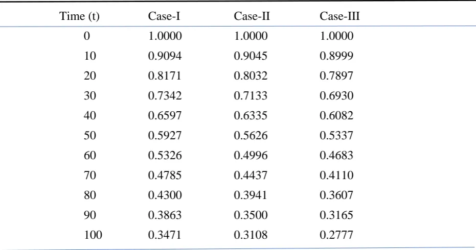
P t with the help of (55-57), as shown in table-2 and figure-2.

Table 2 Variation of availability with respect to time in various cases

Time (t) Case-I Case-II Case-III

0 1.0000 1.0000 1.0000

10 0.9094 0.9045 0.8999

20 0.8171 0.8032 0.7897

30 0.7342 0.7133 0.6930

40 0.6597 0.6335 0.6082

50 0.5927 0.5626 0.5337

60 0.5326 0.4996 0.4683

70 0.4785 0.4437 0.4110

80 0.4300 0.3941 0.3607

90 0.3863 0.3500 0.3165

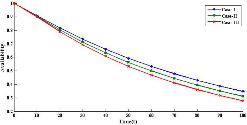
Figure 2 Availability as a function of time

7.2 Reliability Analysis

In order to obtain system reliability, consider repair rates equal to zero. Like availability, the same three cases are discussed here.

Case I: When both the subsystems have a switching device, the reliability of the system by

taking the values of different parameters as

1 2

1 0.03, 2 0.02, s 0.025, s 0.022

 =  =  =  = in (53),

we obtain,

0.1070 0.2370 0.1370 0.1670

0.0670

( )

0.235294

0.012465 t 1.570613 t 0.180000 t 2.142857 t

t

R t e e e e

e

− − − −

−

= +

− + +

(58)

Case II: When subsystem-2 does not have a switching device, the availability of the system by

taking the values of different parameters as

1 2

1 0.03, 2 0.02, s 0.025, s 0

 =  =  =  = in (53), we

obtain,

0.2150 0.1150 0.1450 0.0450

0.0850

( ) 1.570613

0.012462

0.180000 2.142857 0.235294

t t t t

t

R t e e e e

e

− − − −

−

= − +

+ + +

(59)

Case III: When subsystem-1, as well as the subsystem-2, do not have a switching device, the availability of the system by taking the values of different parameters as

1 2

1 0.03, 2 0.02, s 0, s 0

PERFORMANCE ANALYSIS OF A COMPLEX REPAIRABLE SYSTEM

0.1900 0.1200 0.0900 0.0600

0.0200

( ) 1.570613 2.142857

0.235294

0.180000 0.012462

t t t t

t

R t e e e e

e

− − − −

−

= − +

+

+ +

(60)

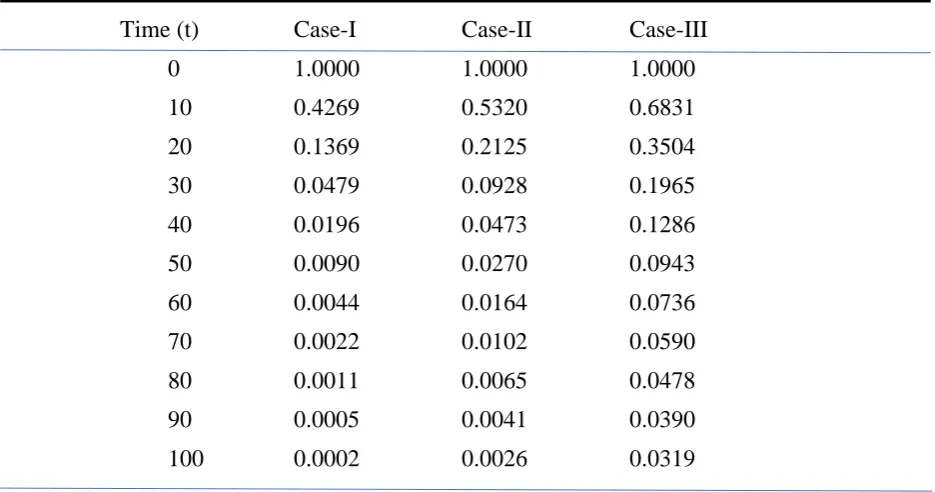
For t=0,10, 20,30, 40,50, 60, 70,80,90 and 100units of time, one may get different values R t( )

with the help of (58-60), as shown in table-3 and figure-3.

Table 3 Computed values of reliability corresponding to the different cases

Time (t) Case-I Case-II Case-III

0 1.0000 1.0000 1.0000

10 0.4269 0.5320 0.6831

20 0.1369 0.2125 0.3504

30 0.0479 0.0928 0.1965

40 0.0196 0.0473 0.1286

50 0.0090 0.0270 0.0943

60 0.0044 0.0164 0.0736

70 0.0022 0.0102 0.0590

80 0.0011 0.0065 0.0478

90 0.0005 0.0041 0.0390

100 0.0002 0.0026 0.0319

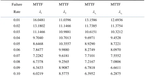
7.3 Mean Time to Failure (MTTF)

Taking all repair rate to zero and the limit as s tends to zero in (53) for the exponential distribution; we can obtain the MTTF as:

2 3

1 1 1 2

1 1 1 2

5 20 60 2

1 1

4 3 2

MTTF    

        

 

= _ + + + + _

+ + + +

  (61)

where

1 2

1 2

5 2 _{s s}

 =  +  + + and

1 2

s s

 = +

Now taking the values of different parameters as

1 2

1 0.03, 2 0.02, s 0.025 and s 0.022

 =  =  =  =

and varying

1 2

1, 2, s and s

    one by one respectively as0.01, 0.02, 0.03, 0.04, 0.05, 0.06, 0.07,

0.08, 0.09, 0.10 in (61), the variation of MTTF, with respect to failure rates, can be obtained in

table-4 and figure-4.

Table 4 Computation of MTTF corresponding to the failure rates

Failure MTTF MTTF MTTF MTTF

Rate ₁ ₂

1

s



2

s



0.01 16.0481 11.0396 13.1586 12.6936

0.02 13.1802 11.1466 11.7385 11.3754

0.03 11.1466 10.9881 10.6151 10.3212

0.04 9.7040 10.7013 9.6971 9.4528

0.05 8.6468 10.3557 8.9290 8.7221

0.06 7.8477 9.9880 8.2749 8.0970

0.07 7.2282 9.6181 7.7101 7.5552

0.08 6.7378 9.2565 7.2167 7.0806

0.09 6.3433 8.9087 6.7818 6.6611

PERFORMANCE ANALYSIS OF A COMPLEX REPAIRABLE SYSTEM

Figure 4 MTTF as a function of failure rates

7.4 Cost Analysis

Let the service facility be always available, then expected profit during 0,t

)

( )

( )

t

p up

E t =K P



For the same set of parameters defined in (53), one can obtain (63). Therefore,

1.1370 2.7829 1.3119 1.0638

1

0.0107 1.1070 1.0670

2

( )

94.57792

{0.002850 0.008099 0.026831 0.092545

94.595676 0.000523 0.088194 }

p

t t t t

t t t

E t K e e e e

e e e K t

− − − −

− −

=

+

− + −

− + + − (63)

Setting K₁=1 K₂ =0.6, 0.5, 0.4, 0.3, 0.2 and 0.1respectively, and varying t=0,10, 20,30, 40,

50, 60, 70,80,90 and 100units of time, the results for expected profit can be obtained as per

Table 5 Profit computation for different values of time

Time

( )

0 0.0000 0.0000 0.0000 0.0000 0.0000 0.0000

10 3.5808 4.5808 5.5808 6.5809 7.5809 8.5809

20 6.2056 8.2056 10.2056 12.2056 14.2056 16.2051

30 7.9551 10.9551 13.9551 16.9551 19.9551 22.9551

40 8.9182 12.9182 16.9182 20.9182 24.9182 28.9182

50 9.1748 14.1748 19.1748 24.1748 29.1748 34.1748

60 8.7966 14.7966 20.7966 26.7966 32.7986 38.7966

70 7.8479 14.8479 21.8479 28.8479 35.8479 42.8479

80 6.3867 14.3867 22.3867 30.3867 38.3867 46.3867

90 4.4649 13.4649 22.4649 31.4649 40.4649 49.4649

100 2.1293 12.1293 22.1293 32.1293 42.1293 52.1293

Figure 5 Expected profit as a function of time

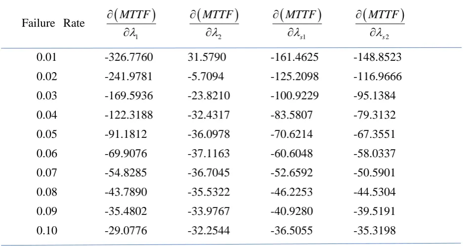
7.5 Sensitivity Analysis corresponding to MTTF

PERFORMANCE ANALYSIS OF A COMPLEX REPAIRABLE SYSTEM

1

1 0.3, 2 0.2, s 0.25

 =  =  = and

2 0.22

s

 = in the partial differentiation of MTTF, one can

calculate MTTF sensitivity, as shown in table-6 and figure-6.

Table 6 MTTF sensitivity as a function of failure rates

Failure Rate

(

)

1

MTTF







(

)

2

MTTF







(

)

1

s

MTTF







(

)

2

s

MTTF



 

0.01 -326.7760 31.5790 -161.4625 -148.8523

0.02 -241.9781 -5.7094 -125.2098 -116.9666

0.03 -169.5936 -23.8210 -100.9229 -95.1384

0.04 -122.3188 -32.4317 -83.5807 -79.3132

0.05 -91.1812 -36.0978 -70.6214 -67.3551

0.06 -69.9076 -37.1163 -60.6048 -58.0337

0.07 -54.8285 -36.7045 -52.6592 -50.5901

0.08 -43.7890 -35.5322 -46.2253 -44.5304

0.09 -35.4802 -33.9767 -40.9280 -39.5191

0.10 -29.0776 -32.2544 -36.5055 -35.3198

8. CONCLUSION

In this paper, the reliability analysis of a complex system consisting of two subsystems, subsystem-1 and subsystem-2 in a series configuration with the switching device, is studied. The subsystems have five and two units, respectively. Furthermore, the switching device in the system is unreliable, and the function of the switch is: "as long as the switch fails, the whole system fails immediately." Using the supplementary variable technique and the Laplace transform various measures like availability of the system, reliability of the system, MTTF, profit analysis, and sensitivity analysis for MTTF are derived in this model.

Table-2 and corresponding figure-2 give the analysis of availability in three different cases on the

switching device. In case I,

1 0.025, 2 0.022

s s

 =  = i.e., both subsystems have a switching device,

in case II,

1 0.025, 2 0

s s

 =  = i.e., only the first subsystem has switching device, while in case III,

1 0, 2 0

s s

 =  = i.e., no subsystem have switching device. It reveals from the graph that availability

constantly decreases as time increases in all the three cases. The reliability of the system is evaluated in three different cases, like availability and shown in table-3 and figure-3. It concludes that reliability decreases significantly in the beginning, and thereafter it decreases approximately in a constant manner. Thus, both the availability and reliability decrease with an increase in time. Investigation through figure 2 and figure 3 concludes that availability values are greater than reliability for the same values of failure rates. Thus, one can understand the need for repair for repairable systems for better performance.

Table-4 and figure-4 yield the MTTF of the system with respect to variation in failure rate

1 2

1, 2, s and s

    , respectively, when other parameters have been kept constant. MTTF of the

system is decreasing concerning different failure rates. MTTF of the system is highest for the failure rate of subsystem-1 and is lowest concerning the failure rate of subsystem-2. The MTTF of switching devices and subsystem-1 are almost the same on failure rate variation value after 0.03.

When revenue cost per unit time fixed atK₁ =1and service costs atK2 =0.6, 0.5, 0.4, 0.3,

0.2 and 0.1, the expected profit has been calculated (Table 5), and the results are demonstrated by the graph (Figure 5). It reveals that expected profit increased as time increased for lower

PERFORMANCE ANALYSIS OF A COMPLEX REPAIRABLE SYSTEM

the profit is higher as compared to the high service cost. The sensitivities of the system MTTF

concerning the system parameter

1 2

1, 2, s and s

    s shown in table-6 and figure-6. The sensitivity

of MTTF for system parameters becomes constant for higher values. Thus, in general, with the study, the behavior of such systems can be analyzed and prognosticate in advance. This paper may be important to engineers, maintenance managers, and plant management for proper maintenance analysis, decision, and for the safety of the system as a whole.

CONFLICT OF INTERESTS

The author(s) declare that there is no conflict of interests.

REFERENCES

[1] A. Khattab, N. Nahas, and M. Nourelfath. Availability of k-out-of-n: G systems with non-identical components subject to repair priorities, Reliab. Eng. Syst. Saf. 94(2)(2009), 142–151.

[2] A. Lado and V.V. Singh. Cost assessment of complex repairable system consisting of two subsystems in the series configuration using Gumbel Hougaard family copula, Int. J. Quality Reliab. Manage. 36(10)(2019), 1683-1698.

[3] A. Munjal and S. B. Singh. Reliability analysis of a complex repairable system composed of two 2-out-of-3: G subsystems connected in parallel, J. Reliab. Stat. Stud. 7(S)(2014), 89-111.

[4] D. Babu, P. Govindaraju, and U. Rizwan. A δ-Shock maintenance model for a deteriorating system with an imperfect delayed repair under partial product process, J. Math. Comput. Sci. 9(5)(2019), 571-581.

[5] Di Bona., G., Forcina, A., Petrillo, A., De Felice, F. A- IFM reliability allocation model based on multicriteria approach. Int. J. Quality Reliab. Manage. 33(5) (2016), 676-698.

[6] Di Bona., G., Forcina, A., Silvestri, A. Critical flow method: A new reliability allocation approach for a thermonuclear system. Quality Reliab. Eng. Int. 32(5)(2016), 1677-1691.

[7] I. Yusuf, and N. Hussaini. A comparative analysis of three redundant unit systems with three types of failures, Arab. J. Sci. Eng. 39(4)(2014), 3337-3349.

[8] I. Yusuf, A, S. Halilu, and N.G. Khalil. Reliability modeling and analysis of a non-repairable series-parallel system, J. Math. Comput. Sci. 6(2) (2016), 247-253.

[9] I. Yusuf, B. Yusuf, and S.I. Bala. Meantime to system failure analysis of a linear consecutive 3-out-of-5 warm standby system in the presence of common cause failure, J. Math. Comput. Sci. 4(1) (2014), 58-66.

[11]K.M. El-Said and M. S. EL-Sherbeny. Evaluation of reliability and availability characteristics of two different systems by using linear first-order differential equations, J. Math. Stat. 1(2)(2005), 119–123.

[12]L. Bulama, I. Yusuf, and S.I. Bala. Stochastic modeling and analysis of some reliability characteristics of a repairable warm standby system, Appl. Math. Sci. 7(2013), 5847-5862.

[13]M. Park and H. Pham. A generalized block replacement policy for a k-out-of-n system with respect to a threshold number of failed components and risk costs, IEEE Trans. Syst. Man Cybern. Part A: Syst. Humans, 42(2)(2012), 453–463.

[14]M. Ram and S. B. Singh. Availability and Cost Analysis of a parallel redundant complex system with two types of failure under preemptive- resume repair discipline using Gumbel-Hougaard family copula in repair, Int. J. Reliab. Quality Safety Eng. 15(4)(2008), 341–365.

[15]N. Goyal, M. Ram M, S. Amoli, and A. Suyal A. Sensitivity analysis of a three-unit series system under k-out-of-n redundancy, Int. J. Quality Reliab. Manage. 34(6)(2017), 770-784.

[16]R. Gupta and A. Tyagi. Stochastic analysis of a two-unit warm standby system with two-phase repair and geometric distributions of the events, J. Math. Comput. Sci. 3(6)(2013), 1586-1600.

[17]R. Gupta, A. Chaudhary, and S. Jaiswal. Stochastic analysis of a three-unit complex system with active and passive redundancies and correlated failures and repair times, J. Math. Comput. Sci. 5 (5)(2015), 694-707. [18]R. Moghaddass, M.J. Zuo, and W. Wang. Availability of a general k-out-of-n: G system with non-identical

components considering shut-off rules using quasi-birth-death process, Reliab. Eng. Syst. Safety, 96(4) (2011), 489–496.

[19]R. Sharma and G. Kumar. Availability improvement for the successive k-out-of-n machining system using standby with multiple working vacations, Int. J. Reliab. Safety, 11(3)(2017), 256-267.

[20]S. C. Malik and S. Deswal. Reliability modeling and profit analysis of a repairable system of non-identical units with no operation and repair in abnormal weather, Int. J. Computer Appl. 51(11)(2012), 43–49.

[21]V. V. Singh, M. Ram, and D. K. Rawal. Cost Analysis of an Engineering System involving subsystems in Series Configuration, IEEE Trans. Autom. Sci. Eng. 10(1)(2013), 1124-1130.

[22]V. V. Singh, S. B. Singh, M. Ram, and C. K. Goel. Availability, MTTF, and cost analysis of a system having two units in a series configuration with the controller, Int. J. Syst. Assur. Manage. 4(4)(2013), 341–352.

[23]V. V. Singh, J. Gulati, D. K. Rawal, and C. K. Goel. Performance analysis of the complex system in the series configuration under different failure and repair disciplines using a copula, Int. J. Reliab. Quality Safety Eng. 23(2)(2016), 1-21.

PERFORMANCE ANALYSIS OF A COMPLEX REPAIRABLE SYSTEM