Workflow Management System for DMS
Nemanja Nedić
1, Goran Švenda
2Faculty of Technical Sciences, University of Novi Sad, Novi Sad, Serbia
e-mail: 1[email protected], 2[email protected]
http://dx.doi.org/10.5755/j01.itc.42.4.
Abstract. Dramatic enrichment of high speed communication technology at affordable costs enabled the resolution of problems related to the limitations of power supply. Therefore, introduction of Smart Grid for managing highly controllable power grids has become indispensable. Its very important part is Distribution Management System (DMS). These sophisticated systems execute a large number of workflows with very high resource requirements. In this paper dynamic, centralized scheduling strategies for allocating DMS workflows are presented and compared. Also, a distributed scheduling algorithm for DMS calculation engine is developed. It is argued that minor investment in the resources and introduction of a hybrid scheduling algorithm leads to the significant boost of the system performance. The hybrid scheduling algorithm is the result of combining centralized and distributed scheduling strategies. Experimental study shows that considerable improvement of overall system performance is achieved by using developed algorithms for designing effective schedulers when make-span and workload are optimized.
Keywords: Smart Grid; Distribution Management System; Workflow Management System; Scheduling; Grid Computing; DAG.
Abbreviations:
CB – Computing Broker
CIM – IEC 61970-301 Common Information Model
CS – Computing Service DAG – Directed Acyclic Graph DDS – Dynamic Data Service
DMS – Distribution Management System DN – Distribution Network
EMS – Energy Management System ESST – Earliest Successors Start Time GDS – Graphical Data Service
SCADA – Supervisory Control and Data Acquisition SDS – Static Data Service
SG – Smart Grid
1. Introduction
Considerable growth of power consumption has been evident in the last two decades [1]. There has been a substantial investment in development of systems for efficient use of energy, which led to reliability increase, power losses reduction and improvement of the environmental protection process. The Smart Grid (SG) is an universal term used to refer to this type of systems [2, 3]. It is a complex collection of
applications which includes subsystems, such as: Supervisory Control and Data Acquisition (SCADA), Energy Management System (EMS), Distribution Management System (DMS), etc.
The DMS [4] is a very important part of the Smart Grid due to its connection to almost all other subsystems. Representation of a distribution network (DN) with a specific data model allows planning, simulation and use of optimization procedures during the real-time control.
Maximal utilization of computational resources and parallelization of independent data processing is necessary to speed up DMS operation. It is possible to divide model data into the groups (partitions) that are independent in terms of calculations [5, 6]. If these fragmented data are processed in parallel, the system performance will be considerably upgraded. Moreover, data import into the DMS is a critical and long-running process. Particularly in cases of invalid import, the process must be repeated to ensure quality data. Most of the input data are not mutually dependent, so the parallel imports are required.
The DMS can rely on the computational Grid technology [7] to store, process and analyze large amounts of distributed data. The Grid computing [8, 9] has moved from academic to commercial domain. Different types of computing offered by the computational Grid provide support for a wide range of rich computation applications [10, 11]. The applications are built for biology [12], physics [13], astronomy [14], etc.
The DMS must become a very powerful high-performance, parallel and distributed application. Therefore, it has to assure the efficient distribution of tasks (which will consider all constraints) over the computational Grid infrastructure.
The computational Grid workload management provides workflow scheduling process that assigns a stream of tasks to available resources in order to optimize various performance metrics. The scheduling strategy can pursue different goals: the fairness of workload distribution, the minimization of workflow execution time, the minimization of a single task execution time, etc. In order to provide fast and reliable response from the computational Grid, scheduling strategies have been intensively studied. Two types of scheduling strategies are thoroughly researched: static [15, 16] and dynamic [15, 17].
A static strategy is used when complete set of tasks is known in advance. Thus, solid estimation of computation cost can be made before actual execution. Scheduling is done prior to the execution of any task.
When tasks are not known prior to the execution, a dynamic strategy is necessary for assigning tasks to resources. Advantage of the dynamic over the static strategy is that the scheduler is aware of run-time behavior of the computational Grid infrastructure. It is useful in a system where the primary goal is maximizing utilization of resources, instead of minimizing execution time of individual task [18].
Since the workflow application is evolving (tasks dynamically arrive, so the application constantly changes) the dynamic scheduling strategy must be considered.
Artificial intelligence, as a modern concept of solving various engineering problems [19, 20], represents a creative approach for workflow schedu-ling. The problems of scheduling that adopt genetic algorithm method for workflow manipulation are addressed in several papers [21, 22]. Since the genetic
algorithm is a static scheduling heuristic, it was necessary to make appropriate adjustments for problems similar to the DMS workflow scheduling. In [23] a dynamic scheduler based on an accommodation of the genetic algorithm for Smart Grid workflows is presented. This approach introduced a number of limitations related to the tasks: tasks must be independent of each other; they must have the same priority and the same execution time. The hierarchical neural networks approach [24] excludes the limitation of tasks having the same execution time, but the restrictions of same priority and independency of tasks remain.
Faced with a variety of situations, an intelligent DMS environment requires complex algorithms which will help to manage the execution of different kinds of workflows. Presented scheduling algorithms consider characteristics of the computational Grid (number and quality of resources) and specific issues of submitted DMS workflows (various execution times, priority of tasks and interdependence between them).
A hybrid algorithm is developed by crossing centralized and distributed scheduling. The centralized scheduling strategy is devoted to global workflow management and monitoring, while the distributed scheduling is adopted for resources that handle the same type of tasks. Each resource that is involved into the distributed scheduling uses smart search to find a partner resource to share a workload. In this way, resources are working cooperatively toward a common goal, and it is easy to include a new resource into the distributed scheduling without any impact on the operation of the centralized scheduling.
A set of the most common DMS workflows is chosen to analyze usability and feasibility of developed schedulers in this field. Two categories of experiments are conducted to simulate the real-world DMS operation: the first category simulates data import into the DMS, while the second category is devoted to the real-time control of a DN.
The developed schedulers are extensively tested and compared. The experimental studies that are carried out confirmed the usefulness of our schedulers when the span [25] is minimized. The make-span of a workflow application is the time interval between the start time of the first task and the completion time of the last task.
2. DMS architecture and computational grid
infrastructure
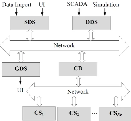
Considering the importance of reliable and efficient operation of the DMS (since it manages the power supply of millions of customers), the deployment of the DMS services is done using dedicated computational Grid resources. Figure 1 presents the core services of the DMS software which are connected by peer-to-peer communication system: • Static Data Service (SDS) provides access to an
a CIM [26] compliant data model which fully describes a power utility DN. After the initial import, these data change very rarely, so it is considered as static data. Most commonly, SDS relies on a relational database which is hosted on the current node.
• Dynamic Data Service (DDS) caches the dynamic states of the devices within a DN. These data are usually received from SCADA system. Since the dynamic state of a DN changes frequently, huge time-series data about process variables must be stored.
• Graphical Data Service (GDS) is responsible for maintaining visual objects that user interface is displaying. This enables each user only to maintain its current view of DN in its memory. As the user moves its view through the DN it can rely on the GDS for the additional graphical data.
• Computing Service (CS) is burdened with the highest requirements. The service provides means for the execution of DMS functions [4]. It receives static and dynamic data for a part of the DN, and performs the requested set of calculations. In respect to the requirements of complicated calculations on large amount of data, CS is deployed on a node with a powerful central processor unit.
Each of these services is deployed on a separate computational Grid node with desired characteristics.
Figure 1. DMS services deployed on a Grid infrastructure The input data of a task need to be stored on a node before processing the task. Since large amount of data is transferred between the DMS services, a suitable mechanism must be used so that data transmission would not represent the bottleneck of the system. A peer-to-peer approach transfers data from a source node to a destination node directly, without involving any third-party service. It reduces transmission time, so it is convenient for large-scale data transfers. To support peer-to-peer communica-tion, every node needs to provide both data management and data movement functionality.
3. DMS workflows
A task is defined as an atomic unit which is executed on a computational Grid resource, and
workflow is a set of tasks with dependencies between them [27]. A workflow can be presented as a directed acyclic graph (DAG) [28,29]. The vertices of the DAG represent the tasks, while the edges are data dependencies between them. Each vertex can have any number of "parent" or "child" vertices. Input tasks of a workflow do not have any "parent" vertices, while output tasks do not have "child" vertices. A task becomes executable when all its dependencies are met (input data required by the task is available at a specified computational Grid resource) and it may be submitted for execution.
By analyzing architecture and requirements of the large- scale distributed DMS, workflows can be presented by the following basic types:
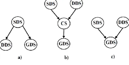
• Model Update is a set of tasks that needs to be executed when a request for the static data update arrives to the system (Figure 2a). Based on the modification of static model, it is necessary to update graphical model and dynamic model. This workflow is common during the initial data import, but it is rare in everyday operation of the system.
• DMS Function Execution is usually triggered by the SCADA system (Figure 2b). When a dynamic state of a device occurs, the part of dynamic data model and correspondent static data model are transferred to the CS. The relevant calculations on data are performed and graphical data model is updated with results. During the everyday operation of the system this set of tasks is the most frequent.
• Graphical View Refresh is usually executed periodically, or as a possible error recovery of the GDS (Figure 2c). The part of static data and correspondent dynamic data are transferred to the GDS and graphical data model is updated (refreshed). This workflow is quite rarely executed.
Workload of each task can be evaluated from the historical data [30], and it is easy to know a computing capacity of a resource by knowing its characteristics. Therefore, an estimation of a task execution time is easily determined by dividing the workload of the task with the computing capacity of the resource.
The workflows that arrive to the system are ranked by the priority, and all tasks contained by a workflow obtain the same priority as the workflow.
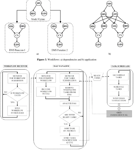
During the further analysis of the system operation, it becomes obvious that there are dependences between the entire workflows that arrive for execution. Figure 3a presents a typical sequence of workflows execution; a data import must precede the execution of DMS functions on the imported data. Figure 3b shows how a workflow application is built. Output tasks of the "parent" workflow become predecessors for the input tasks of the "child" workflow.
Based on the previous discussion, the main properties of a task 𝑇 are: the priority – 𝑝 , the estimated time to execute task – 𝑡 (which corresponds to the estimated task workload – 𝑤), the execution node (DMS service) – ni, ni{SDS,GDS,DDS,CS}. Sets of predecessor tasks and successor tasks of the task 𝑇 are defined by PTi and STi , respectively. Scheduling algorithms use these properties for optimal allocation of resources for task execution. Optimiza-tion goal is to rearrange incoming workflow tasks in order to support the priority and get maximum usage of all nodes, so that the make-span is minimized.
Figure 3. Workflows: a) dependencies and b) application
4. Workflow management system
The Workflow Management System takes into account the dynamic nature of a real-world DMS and uses the computational Grid environment approach for detecting and responding to changes in the DMS. The developed framework is presented in Figure 4. It provides required support for the high-throughput scheduling process.
The framework consists of three components: the Workflow Receiver, the DAG Manager, and the Task Scheduler.
The Workflow Receiver accepts workflows in run time and validates for appropriate workflow pattern [27]. If a workflow is valid, it is sent to the DAG Manager, otherwise it is rejected.
The DAG Manager controls the workflow application. The workflow application is represented via a DAG and it is continually evolving during the system operation. The DAG Manager monitors the incoming workflows and task completion events. When any of the events occur, the DAG is updated: a new, valid workflow is included, while the completed task is removed from the workflow application. The dependency information is updated. When the DAG modification is finished, determination which tasks have become suitable for execution based on dependencies in the workflow is started. The result of analysis is a list of executable tasks. It contains tasks that have no predecessors. The list of executable tasks is partitioned into the levels. The tasks with same priority are classified within the same level. The levels are sorted in descending order by priority and tasks organized in this manner are submitted for scheduling. The Task Scheduler is responsible for resource selection and mapping tasks to resources. This component is of the most interest in our research, since the decision making is done in it. The scheduler maintains a task queue which is constantly read. The tasks are independent and classified to levels by priority. The level by level methodology considers tasks at the current level. The tasks from the highest priority level are collected and scheduling algorithm is applied to determine the right time to send tasks for execution. After that, it is moved to a lower priority level, and so forth. Depending on the specific characteristics of the computational Grid infrastructure and task properties, different scheduling algorithms can be deployed on the Task Scheduler.
5. Workflow application model
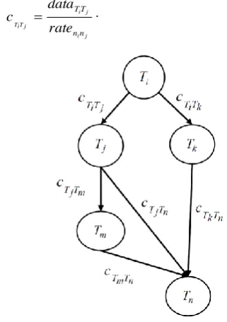
As outlined above, the workflow application is represented with a DAG. The tasks without any predecessors are input tasks, while the tasks without any successors are output tasks (Figure 5).
A task Ti is defined as a triple:
i n t p
Ti ( i, i, i), , (1)
where 𝑝 is task priority, 𝑡is estimated time to execute task (corresponding the estimated task workload –𝑤), and 𝑛 is execution node (DMS service).
The computational Grid infrastructure is fully connected topology in which communications are performed without any constraints. It is assumed that data transfer rates (amount of data that can be transferred) between nodes are known. Transfer rate between nodes 𝑛 and 𝑛 is denoted by rateninj . Amount of data that needs to be transferred after completion of task 𝑇 and before start of task 𝑇 is denoted by dataTiTj . Finally, communication time cost of edge (𝑖, 𝑗) is defined as:
j i
j i
j T i T
n n
T T
rate data
c . (2)
Figure 5. Workflow application model
Let us define 𝑠𝑡 and 𝑐𝑡 as start time and completion time of a task 𝑇, respectively, and ntni as the earliest available time of a node 𝑛. To determine when the task 𝑇 has become eligible for execution all predecessors of that task must be scheduled:
j TiTj i
i T j
i T P T n
T ct c nt
st max max{ }, , (3)
where PTi is a set of predecessor tasks of task 𝑇. The completion time ctTi is calculated as the sum of
i T
st and the estimated execution time 𝑡 of task 𝑇:
i Ti
T
st
t
ct
i
. (4)The make-span of the workflow application is time period taken from the start of the application, up until all outputs are available:
} { max
i i
T Outputs
T ct
makespan
. (5)
6. Centralized scheduling architecture
As the set of workflows that should be executed on the computational Grid is not known in advance, but workflows arrive continuously, all information regarding the tasks is not entirely known before execution time. Therefore, scheduling decisions must be made on the fly, and the dynamic scheduling algorithms are necessary. The Task Scheduler contains executable, independent tasks categorized by priority levels. The scheduling algorithms consider tasks level by level, starting from the level with the highest priority.
1. Earliest successors start time algorithm (ESSTA)
The algorithm is based on the idea of primary scheduling tasks that will lead to the possibility of executing all its successors in the shortest period of time. The question that is answered is: which of the executable tasks need to be completed to enable scheduling of all its successors as soon as possible?
The 𝑠𝑢𝑐𝑐𝑠𝑡 is defined as estimated time when all the successors of a task 𝑇 are ready for the execution:
}
{
max
j T i T i T j i
i
ct
c
succst
S T T
T
. (6)The algorithm considers all unmapped tasks within a priority level during each scheduling decision. It schedules tasks in order that changes the node availability status. Listing 1 shows the pseudo code for EEST algorithm:
for all (priorityLevelsortedTasksPiorityLevels)
while (TpriorityLevel is not scheduled) ue someMaxVal mum
succstMini
emptyTask ute
taskToExec
0 index
for all (TipriorityLevel)
compute succstTi
if (succst succstMinimum
i
T )
i T
succst mum
succstMini
i
T ute taskToExec
i index
end if end for all
schedule taskToExecute
remove taskToExecute from vel
priorityLe
update ntnindex
end while end for all
Listing 1.Earliest successors start time algorithm
The algorithm schedules a set of independent tasks iteratively. For each iteration, it computes succst for every task. A task having minimum succst value is chosen to be scheduled first and it is assigned to the appropriate resource. The expectation is that a smaller make-span can be obtained if tasks assigned to resources allow their successors to enter the scheduling process more quickly.
2. Critical path algorithm (CPA)
The algorithm relies on the concept of the workflow application critical path [31, 32]. The critical path approach aims to determine the longest of all execution paths from the beginning to the end in a DAG. It answers the question: which tasks have the most impact on the overall execution time? The algorithm captures tasks (within the priority level) that block the most time-consuming activities in the workflow application and schedule them earliest to minimize execution time for entire DAG.
The tasks within the same priority level are ordered by their rank (critical path value). The rank of output tasks corresponds to their execution time:
i Outputs T
T t rank
i i
. (7)
The ranks of other tasks are calculated recursively:
} {
max j
j T i T i T j
i i T S T
T t c rank
rank
, (8)
where 𝑆 is the set of all successors of the task 𝑇. A task with higher rank value is given earlier execution time. The pseudo code for critical path algorithm is presented in Listing 2:
for all (priorityLevelsortedTasksPiorityLevels)
while (TpriorityLevelis not scheduled) 0
m rankMaximu
emptyTask ute
taskToExec
0 index
for all (TipriorityLevel)
computerank Ti
if (rankTi rankMaximum)
i
T
rank m rankMaximu
i
T ute taskToExec
i index
end if end for all
scheduletaskToExecute
remove taskToExecute from vel
priorityLe
update ntnindex
end while end for all
3. Experiments and results
A distributed testing environment based on the proposed architecture is developed to simulate the real-world DMS operation. Intel Core i3 (3.30 GHz) microprocessors are assigned to each node and computer devoted to workflow management. All software components are implemented in .NET 4.0 framework. Performed experiments are classified into two categories: data import and real-time control.
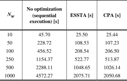
The first set of experiments simulates data import into the system. This kind of work is usually done offline, before real-time control of a DN starts. The workflow application is designed only of Model Update workflows. Number of workflows (Nw) that dynamically arrive for execution varies depending on the number of entities which have to be imported into the system. The number of entities is within the range from a few thousands to several millions; therefore, it is used between ten and a thousand workflows in our experiments. Table 1 and Figure 6 summarize results of scheduling comparison.
The second set of experiments is devoted to the simulation of real-time control of a DN. The workflow application is composed of all three types of workflows. The DMS Function Execution is the most common and represents more than 70% of all workflows that arrive for execution. The Model Update workflow type makes about 20% of the workflow application, while the Graphical View Refresh type is the rarest (up to 10%). Similar to the first set of experiments, it is used between ten and a thousand workflows. Obtained results are presented in Table 2 and Figure 7.
All experiments examine the effect of make-span changes. The developed algorithms are compared to the sequential approach of task manipulation. As expected, by introducing parallelization of tasks and dynamic schedulers into the operation of a large scale DMS, the essential improvement of computational resources exploitation is provided.
Table 1.Workflows execution time – DMS data import
Nw
No optimization (sequential execution) [s]
ESSTA [s] CPA [s]
10 45.70 25.50 25.44
50 228.72 108.53 107.23
100 456.52 208.54 206.50
250 1154.37 522.77 513.87
500 2288.11 1048.65 1026.14
1000 4572.27 2075.71 2050.68
Figure 6. DMS data import - Workflows execution Table 2.Workflows execution time – DMS real-time control
Nw
No optimization (sequential execution) [s]
ESSTA [s] CPA [s]
10 62.03 36.89 34.05
50 310.35 148.01 146.33
100 618.62 293.37 288.58
250 1546.19 729.05 723.41
500 3093.00 1452.24 1442.90
1000 6192.01 2906.62 2881.85
Figure 7. DMS real-time control - Workflows execution 0
500 1000 1500 2000 2500 3000 3500 4000 4500
10 50 100 250 500 1000
E
x
ec
u
ti
o
n
t
im
e
[s]
Number of workflows
DMS Data import - Workflows execution time
No optimization ESSTA CPA
0 1000 2000 3000 4000 5000 6000
10 50 100 250 500 1000
E
x
ec
u
ti
o
n
t
im
e
[s]
Number of workflows
DMS real-time control - Workflows execution time
Based on illustrated experimental results the following can be noted:
• The CPA based scheduler outperforms the ESSTA solution. Explanation for this phenomenon can be found in fact that the CPA considers all execution paths, while the ESSTA analyzes only a close environment of a task in the DAG.
• The scheduling brings more benefits if there are more tasks to rearrange.
• The performance of the system improves with increase of the number of workflows.
7. Hybrid scheduling architecture
During the real-time system operation, DMS Function Execution is by far the most frequent type of workflow that arrives for execution. Taking into account the processing of large amount of data within this workflow type, the computing node (CS, Figure 1) is heavily loaded. Therefore, it represents the bottleneck of the system. Introduction of additional computing nodes into the computational Grid infrastructure would allow the possibility of supplementary workload distribution.
Figure 8 presents the improvement of computational Grid infrastructure for developed hybrid scheduling algorithm. More advanced computing engine includes multiple computing nodes and establishes the Computing Broker (CB) node. The computing nodes implement a distributed scheduling algorithm [33], while the CB represents a mediator between them and the other parts of the system. The Workflow Management System schedules computing tasks and data needed for their execution to the CB. When a computing node adopts a task, it takes data contained by the CB and executes expected calculation. After completing the task, the computing node transfers results to the CB, which forwards them to the appropriate node and notifies the Workflow Management System of the task completion.
Figure 8. Grid infrastructure for hybrid scheduling
1. Distributed scheduling algorithm
The main aim of distributed computing is to achieve parallelism through the workload distribution and obtain better execution time. Capabilities of the computing nodes may be different because of their heterogeneous computation power. In order to efficiently use computing nodes it is necessary to assign workload proportionally to their computation power. With the purpose of simplifying the explanation of our solutions, the distributed dynamic algorithm is presented for the computing nodes with homogeneous computation power. It is very easy to adapt it to a set of computing nodes with various computation capacities.
The workload of a node ni is defined as nwni. 𝑁𝐶 is the set of all computing nodes within a computational Grid infrastructure. Its cardinality is denoted by 𝑁. The purpose of scheduling process is to make workload distribution system converge towards the desired workload distribution:
NC n nw
nwn i
i , . (9)
nw is the workload that every computing node should receive. Because the system is assembled of the computing nodes with homogeneous computation power, nw is defined as:
c NC n
n
N nw
nw i
i
. (10)
The distributed dynamic algorithm is run during the tasks execution and allows us to adapt workload distribution as the executions proceed. It is based on the physical phenomenon of diffusion. The iterative diffusion algorithm makes decisions about workload balancing at the iteration ℎ by using the workload information of the previous iteration ℎ − 1 [34]. At iteration ℎ the workload of a node 𝑛 is represented as
h ni
nw . According to the diffusion iterative algorithm
the computing node ni exchanges the portion of
workload h
n h
ni nw j
nw
with a computing node
𝑛 at each iterative step. Parameter 𝛼 determines how much of workload difference will be exchanged and depends on the considered problem [34,35]. Workload transformation of the computing node ni is described by the following equations:
NC n
h n h n h
n h n
j
i j i
i nw nw nw
nw 1 [ 1 1], (11)
NC n
h n h
n c h
n
j
j i
i N nw nw
nw [1 ] 1 1. (12)
workload balance is presented by some norm, for example quadratic
NC n n i i nw
nw ]2
[ . In [34] it is
proved that this algorithm converges towards the uniform workload distribution.
2. Accommodation of distributed scheduling algorithm
As explained above, in distributed algorithm it is assumed that it is possible to exchange any portion of workload between nodes. That is, the workload portion is a continuous value. In practice, the situation is somewhat different. A set of tasks is assigned to each computing node. It is possible to distribute only complete tasks between nodes, so the portion of workload for exchange takes discrete values. Parameter determines the amount of workload exchange, and consequently the algorithm convergence speed and quality. To achieve the highest possible workload sharing between nodes, the parameter 𝛼 is set to 1 / 2 (𝛼 = 1/ 2).
i n
TC is defined as a set of computing tasks that are assigned to the computing node 𝑛 and whose execution didn’t start. nwninj is the maximum amount of workload that the computing node 𝑛 can exchange with a computing node 𝑛:
]
[ i j
j
in n n
n nw nw
nw
. (13)
j in n
TC
is a subset of tasks adopted by the computing node 𝑛 (subset of
i
n
TC ) for which the overall sum of workloads has a maximum value:
j n i n k i n j n in T TC
k TC Pow TC w ( )
max , (14)
but with a constraint that the overall sum of workloads does not exceed nwninj :
j i j n i n k n n TC T k nw w
. (15)
) (TCni
Pow represents the power set of i
n
TC (the set of all subsets of TCniincluding the empty set).
If h n ni j
is determined as the portion of workload that will be exchanged between nodes 𝑛 and 𝑛 at the iterative step ℎ, then evolution of the computing nodes workload is calculated according to the following rules:]
[ 1 1
1
h
n h
n h
n
ni j nw i nw j
nw
(16) 1 1 1 1 ,
h TC T k h n h j n i n h j n i n k i j n in TC w nw
TC (17)
1 1 h j n i n k j i TC T k h n n w (18) 1 1 h n n h n hni nw i i j
nw
(19)1 1 h n n h n h
nj nw j i j
nw
(20)1
1\
h h
n h
ni TC i TCninj
TC (21)
1 1 h n n h n h
nj TC j TC i j
TC
(22)The algorithm is completed when workload is balanced in such a manner that there is no need for further exchange. This is achieved when h
n ni j TC
becomes an empty set of tasks for every possible combination (𝑖, 𝑗) . This is equivalent to
) , ( , 0 i j h
n
ni j
. Listing 3 clarifies the algorithm for distributed scheduling:while( finished true)
// assuming that algorithm is finished true
finished
for all (niNC)
for all (njNC)
computenwninj
determine j in n TC
if (TCninj not empty)
computeninj
j i i
i n nn
n nw
nw
j i j
j n nn
n nw
nw
j i i
i n nn
n TC TC
TC \
j i j
j n nn
n TC TC
TC
// algorithm is not finished false finished
end if end for all end for all end while
Listing 3.Distributed scheduling algorithm
It should be emphasized that the tasks are organized by priority within each computing node, so the tasks that are more important are executed first.
3. Experiments and results
of the DMS real-time control of a DN. The Task Scheduler operates according to the critical path algorithm, while the computing nodes use the distributed algorithm for redistributing computing workload. The same set of tests for examination of centralized scheduling algorithms is used.
In the first experiment, the computing engine contains three computing nodes. Table 3 presents the results of scheduling comparison.
Table 3. Workflows execution time – Hybrid scheduling
Nw ESSTA [s] CPA [s] Hybrid scheduling [s]
10 36.89 34.05 27.87
50 148.01 146.33 84.75
100 293.37 288.58 155.26 250 729.05 723.41 371.45
500 1452.24 1442.90 732.15
1000 2906.62 2881.85 1445.92
The quality of results produced by the hybrid scheduler is compared to the results reported for the centralized scheduling algorithms (Figure 9).
Figure 9. DMS real-time control – Hybrid scheduling workflows execution
The experimental study leads to the following conclusions:
• The hybrid scheduling algorithm significantly outperforms previous (centralized) solutions. • The performance (specifically, the speed) increases
by increasing the number of workflows.
• A minor investment into the computational Grid resources and deployment of the hybrid scheduling architecture solves computing bottleneck of the large scale DMS.
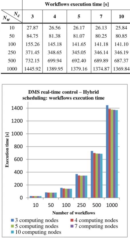
• Introduction of the dynamic hybrid scheduler into the task scheduling process provides considerable improvement of resources exploitation which results in better performance of the entire system. The second experiment is devoted to dependency between the system performance and a number of computing nodes within the computing engine. Table 4 and Fig. 10 present the acquired results.
Table 4.Workflows execution time – Hybrid scheduling with different number of computing nodes
Workflows execution time [s]
Nw Nc 3 4 5 7 10
10 27.87 26.56 26.17 26.13 25.84 50 84.75 81.38 81.07 80.25 80.85
100 155.26 145.18 141.65 141.18 141.10 250 371.45 348.65 345.05 346.14 346.19
500 732.15 699.94 692.40 689.89 687.37
1000 1445.92 1389.95 1379.16 1374.87 1369.84
Figure 10. DMS real-time control – Hybrid scheduling workflows execution with different number of computing
nodes
According to the experimental results, it is concluded:
• By increasing the number of the computing nodes the system performance increases, but progression is not proportional to the number of computing nodes.
• After reaching a certain number of the computing nodes the saturation occurs.
0 500 1000 1500 2000 2500 3000
10 50 100 250 500 1000
E
x
ec
u
ti
o
n
t
im
e
[s]
Number of workflows
DMS real-time control - Hybrid scheduing: workflows execution time
ESSTA CPA Hybrid algorithm
0 200 400 600 800 1000 1200 1400
10 50 100 250 500 1000
E
x
ec
u
ti
o
n
t
im
e
[s]
Number of workflows
DMS real-time control – Hybrid scheduling: workflows execution time
• Investment into the computing engine is justified only if there is significant boost of the system performance.
8. Conclusion
The suggested Workflow Management System considers dynamic nature of the large scale DMS and supports high-throughput scheduling. Different dynamic scheduling strategies which maintain workflows priority and dependency have been developed and discussed.
Two centralized strategies for maximizing system utilization are developed: the earliest successors start time and the critical path algorithms. By engaging these algorithms, the crucial progress in the computational resources utilization is produced. Experimental studies presented usefulness of these algorithms. The studies show a slight advantage of the critical path algorithm. The advantage of the centralized strategies is easy implementation, however, they lack scalability.
Further analysis of the DMS operation in real-time control mode revealed that it is necessary to provide additional support to heavily loaded computing node. Suggested solution provides an advanced computing engine with multiple computing nodes which implement the designed distributed workload balancing. In this way, the hybrid scheduling architecture is achieved. The aim of presented experimental study is to reveal effectiveness of the hybrid based scheduling. The performance analysis shows that this approach significantly reduces the total execution time and boosts the performance of the whole system.
References
[1] F. P. Sionsansi. Smart Grid: Integrating Renewable, Distributed & Efficient Energy. Academic Press, 2011. [2] E. Santacana, G. Rackliffe, L. Tang, X. Feng.
Getting Smart. IEEE Power and Energy Magazine, 2010, Vol. 8, No. 2, 41-48.
[3] A. Bose. Smart transmission grid applications and their supporting infrastructure. IEEE Trans. on Smart Grid, 2010, Vol. 1, No. 1, 11-19.
[4] D. S. Popović. Power applications: A cherry on the top of the DMS cake, DA/DSM DistribuTECH Europe, Vienna, Austria, 2000.
[5] D. Capko, A. Erdeljan, M. Popovic, G. Svenda. An optimal initial partitioning of large data model in utility management systems. Advances in Electrical and Computer Engineering, 2011, Vol. 11, No. 4, 4146.
[6] D. Capko, A. Erdeljan, S. Vukmirovic, I. Lendak. A hybrid genetic algorithm for partitioning of data model in distribution management systems. Information Technology and Control, 2011, Vol. 40, No. 4, 316322.
[7] I. Foster, C. Kesselman, S. Tuecke. The anatomy of the grid: enabling scalable virtual organization.
International Journal of Supercomputer Applications, 2001, Vol. 15, No. 3, 200-222.
[8] A. Kaceniauskas, R. Pacevic, A. Bugajev, T. Katkevicius. Efficient visualization by using Paraview software on Baltic grid. Information Technology and Control, 2010, Vol. 39, No. 2, pp. 108-115.
[9] A. Kaceniauskas. Solution and analysis of CFD applications by using grid infrastructure. Information Technology and Control, 2010, Vol. 39, No. 4, 284290.
[10] D. Abramson et al. Deploying scientific applications to the PRAGMA grid testbed: strategies and lessons. In: Sixth IEEE International Symposium on Cluster Computing and the Grid, Washington, DC, USA, 2006, pp. 241-248.
[11] G. Allenet al. GridLab: enabling applications on the Grid. In: GRID ’02: Third International Workshop on Grid Computing, London, UK, 2002, pp. 39-45. [12] E. Deelmana et al. Pegasus: mapping scientific
workflows onto the grid. In: 2-nd European Across Grids Conference, Nicosia, Cyprus, 2004, pp. 11-20. [13] E. Deelman et al. GriPhyN and LIGO, building a
virtual data grid for gravitational wave scientists. In: 11-th Intl. Symposium on High Performance Distributed Computing, Edinburgh, Scotland, 2002, pp. 225-234.
[14] G. B. Berrimanet al. Montage: a grid enabled image mosaic service for the national virtual observatory. In: Astronomical Data Analysis Software and Systems XIII, Strasbourg, France, 2003, pp. 593-596.
[15] H. J. Siegel, S. Ali. Techniques for mapping tasks to machines in heterogeneous computing systems. Journal of Systems Architecture, 2000, Vol. 46, 627639.
[16] T. D. Braun et al. A comparison study of static mapping heuristics for a class of meta-tasks on heterogeneous computing systems. In: Heterogeneous Computing Workshop, San Juan, Puerto Rico, 1999, pp. 15-29.
[17] M. Maheswaran, S. Ali, H. J. Siegel, D. Hensgen, R. F.Freund. Dynamic mapping of a class of independent tasks onto heterogeneous computing systems. Journal of Parallel and Distributed Computing, 1999, Vol. 59. No. 2, 107131.
[18] H. A. James. Scheduling in Metacomputing Systems, Ph.D. Thesis. The Department Of Computer Science, University of Adelaide, Australia, 1999.
[19] A. Gokhan Ak, G. Cansever, A.Delibasi. Robot trajectory tracking with adaptive RBFNN-based fuzzy sliding mode control. Information Technology and Control, 2011, Vol. 40, No. 2, 151156.
[20] A. Kuczapski, M. V. Micea, L. A. Maniu, V. I. Cretu. Efficient generation of near optimal initial populations to enhance genetic algorithms for job-shop scheduling. Information Technology and Control, 2010, Vol. 39, No. 1, 32-37.
[21] V. Di Martino, M. Mililotti. Sub optimal scheduling in a grid using genetic algorithms. Parallel Computing, 2004, Vol. 30, 553-565.
[23] N. Nedic, S. Vukmirovic, A. Erdeljan, L. Imre, D. Capko. A genetic algorithm approach for utility management system workflow scheduling. Information Technology and Control, 2010, Vol. 39, No. 4, 310316.
[24] S. Vukmirovic, A. Erdeljan, I. Lendak, D. Capko, N. Nedic. Optimization of workflow scheduling in Utility Management System with hierarchical neural network. International Journal of Computational Intelligence Systems, 2011, Vol. 4, No. 4, 672-679. [25] M. Iverson, F. Ozguner. Dynamic, competitive
scheduling of multiple DAGs in a distributed heterogeneous environment. In: Heterogeneous Computing Workshop, Orlando, Florida, USA, 1998, pp. 70-78.
[26] IEC 61970 Energy management system application program interface (EMS-API) – Part 301: Common Information Model (CIM) Base, IEC, Edition 2.0, 2007.
[27] W. M. P. van der Aalst, A. H. M. ter Hofstede, B. Kiepuszewski, A. P. Barros. Workflow patterns. Technical Report, Eindhoven University of Technology, 2000.
[28] R. Sakellariou, H. Zhao. A low-cost rescheduling policy for efficient mapping of workflows on grid systems. Scientific Programming, 2004, Vol. 12, No. 4, 253-262.
[29] T. Tannenbaum, D. Wright, K. Miller, M. Livny.
Condor: a distributed job scheduler, Beowulf cluster computing with Linux. The MIT Press, MA, USA, 2002.
[30] S. Hotovy. Workload evolution on the Cornell theory center IBM SP2. In: Workshop on Job Scheduling Strategies for Parallel Processing, Honolulu, Hawaii, USA, 1996, pp. 27-40.
[31] H. Topcuoglu, S. Hariri, M. Y. Wu. Performance-effective and low-complexity task scheduling for heterogeneous computing. IEEE Trans. on Parallel and Distributed Systems, 2002, Vol. 13, No. 3, 260274.
[32] J. H. Son, M. H. Kim. Analyzing the critical path for the well-formed workflow schema. In: International Conference on Database Systems for Advanced Applications, Hong Kong, China, 2001, pp. 146-147. [33] M. Arora, S. K. Das, R. Biswas. A decentralized
scheduling and load balancing algorithm for heterogeneous grid environments. In: International Conference on Parallel Processing Workshops, Vancouver, Canada, 2002, pp. 499-505.
[34] G. Cybenko. Dynamic load balancing for distributed memory multiprocessors. Journal of Parallel and Distributed Computing, 1989, Vol. 7, No. 2, 279-301. [35] C. Xu, F. Lau. Optimal parameters for load balancing
with the diffusion method in mesh networks. Parallel Processing Letters, 1994, Vol. 4, No. 2, 139-147.
Received June 2013.
Appendix – Example of distributed scheduling
A simplified example of a workload distribution is introduced in this section. Workload of a computing task is represented via an integer value. Execution did not start for any of the tasks. The computing engine includes three computing nodes; total workload of the first node is 14, 10 of the second node, and 4 of the third (Fig. 11). The parameter 𝛼 is set to 1 / 2 (𝛼 = 1/ 2).4
3
3
2
2 = 14
4
3
2 1 = 10
2
2 = 4
n
1:
n
2:
n
3:
Figure 11. Initial workload state of the computing nodes The first iteration starts with transferring tasks form node 𝑛 to other nodes. Maximum allowed amount of workload that may be transferred is calculated, but actual workload portion for exchange is based on the set of tasks which are located at the first node. Fig. 12 shows the exchange of a task between nodes 𝑛 and 𝑛 , and the resulting values of total workload for nodes.
14 10
2 5. 0
1 2
1
nwnn
2
1 2 1n
n
4
3
3
2
2
4
3
2
n
1:
n
2:
2 1 = 12
= 12
Figure 12. Transferring task with workload value equal 2 from node n1 to node n2
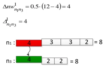
Similarly, the workload exchange takes place between nodes 𝑛 and 𝑛 : when values nw13 and
13
are determined, a task is transferred (Fig. 13).
12 4
45 . 0
1 3
1
nwnn
4
1 3 1n
n
4
3
3
2
2
2 = 8
n
1:
n
3:
= 8
4
Fig. 14 presents the new distribution of workload after tasks are transferred from node 𝑛 to other nodes.
3
3
2 = 8
4
3
2
1 = 12
2
2 = 8
n
1:
n
2:
n
3:
4
2
Figure 14. Workload state of the computing nodes after transmission of tasks form node 𝑛 at the first iteration
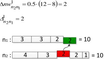
The next step at the first iteration is the workload exchange between node 𝑛 and remaining nodes. The exchange starts with node 𝑛 (Fig. 15).
12 8
2 5. 0
1 1
2
nwn n
2
1 1 2n
n
3
3
2
= 10
4
3
2
1 = 10
n
1:
n
2:
2
2
Figure 15. Transferring task with workload value equal 2 from node 𝑛 to node 𝑛
The principle is the same as for the previous step (Fig. 16).
10 8
1 5. 0
1 3
2
nwn n
1
1 3 2n
n
4
3
1 = 9
2
2
= 9
n
2:
n
3:
4
2
1
Figure 16. Transferring task with workload value equal 1 from node n2 to node n3
Fig. 17 presents the new distribution of workload after tasks are transferred from node 𝑛 to other nodes.
3
3
2
= 10
4
3
= 9
2
2
= 9
n
1:
n
2:
n
3:
4
2
2
1
Figure 17. Workload state of the computing nodes after transmission of tasks form node n2
The workload of node 𝑛 is less or equal than the workload of remaining nodes, therefore there will be no workload sharing.
9 10
0 5. 0
1 1
3
nwnn
0
1 1 3n
n
9 9
0 5. 0
1 2
3
nwnn
0
1 2 3n
n
The second iteration begins the same as the first, by exchanging the workload of node 𝑛 with other nodes. The workload difference is not big enough, so there is no exchange.
2 1 9 10 5 . 0 2 21
nwnn
0
2 2 1n
n
2 1 9 10 5 . 0 2 31
nwnn
0
2 3 1n
n
The amount of workload at node 𝑛 is also not big enough to make an exchange with other nodes.
9 10
0 5. 0
2 1
2
nwn n
0
2 1 2n
n
9 9
0 5. 0
2 3
2
nwn n
0
2 3 2n
n
The same situation applies to node𝑛 .
9 10
0 5. 0
2 1
3
nwnn
0
2 1 3n
n
9 9
0 5. 0
2 2
3
nwnn
0
2 2 3n
n
Since the completion condition is met:
1,2,3
1,2,3
),, ( ,
0
i j i j
j in n
,