Volume 13 - Article 21 | Pages 547–558

Demographic Research a free, expedited, online journal of peer-reviewed research and commentary

in the population sciences published by the Max Planck Institute for Demographic Research Konrad-Zuse Str. 1, D-18057 Rostock · GERMANY www.demographic-research.org

DEMOGRAPHIC RESEARCH

VOLUME 13, ARTICLE 21, PAGES 547-558

PUBLISHED 22 NOVEMBER 2005

http://www.demographic-research.org/Volumes/Vol13/21/ DOI: 10.4054/DemRes.2005.13.21

Research Article

Five period measures of longevity

John Bongaarts

1 Introduction 548 2 Definitions of period longevity measures 548

3 Results 550

4 Discussion 554

5 Conclusion 555

6 Acknowledgments 556

Demographic Research: Volume 13, Article 21 a research article

Five period measures of longevity

John Bongaarts 1

Abstract

This study provides a summary of recently proposed alternatives period measures of "longevity" and assesses whether empirical differences between these measures are consistent with predictions from analytic studies. Particular attention is given to the tempo effect. Three of the five period measures are virtually equal to one another in a simulated population in which mortality follows a Gompertz model with a constant rate of improvement. Similar results are observed among females in Denmark, England and Wales and Sweden in the last quarter century. However, these three measures differ substantially from the conventional period life expectancy when mortality changes over time. These findings are consistent with theoretical analysis by Bongaarts and Feeney (2002, 2003, 2005) which demonstrated that this deviation is caused by a tempo effect whose size varies with the rate of change in mortality.

1. Introduction

The most widely used measure of period mortality is life expectancy at birth calculated with a conventional life table. Alternative period measures of “longevity” exist, but have found very limited application. The purpose of this note is to provide a brief summary of recently proposed alternatives and to assess whether empirical differences between these measures are consistent with predictions from analytic studies. Particular attention will be given to the tempo effect as a cause of differences between measures. Comparisons rely on simulations in which the force of mortality follows a Gompertz model with a constant rate of improvement over time. Empirical estimates are also provided for three countries with long historical data series. A brief concluding comment summarizes the main reasons why certain measures differ and why others are nearly the same.

2. Definitions of period longevity measures

1) Life expectancy

∫

∫

∞

− =

0 0

0() exp{ ( , ) }

x dx da t a t

e µ (1)

where µ(a,t) is the force of mortality at age a and time t. Standard demographic text books (e.g. Preston et al. 2001) discuss the calculation of this conventional measure. Estimates of e0 are available for most countries of the world (United Nations, 2003)

2) Cross-sectional average length of life (Brouard 1986, Guillot, 2003)

∫

(t p at ada

CAL c (2)

where pc (a,t – a) equals the proportion of survivors at age a and time t for the cohort

Demographic Research: Volume 13, Article 21

3) Tempo adjusted life expectancy (Bongaarts and Feeney 2003; Vaupel, 2005)

∫

∫

e µ (3)

This is a variant of the conventional period life expectancy, but the tempo effect in the force of mortality is removed by dividing this rate by 1 – r(t). The variable r(t), which is assumed to be the same for all ages, denotes the increments to life (or the delay in deaths) due to mortality improvements at time t. Vaupel (2005) refers to e0*(t) as the “true life expectancy.” Bongaarts and Feeney (2003) estimate r(t) as

dt t dCAL t

r()= () (4)

This estimate holds in populations in which the function pc (a,t – a) shifts to higher

and lower ages over time while maintaining its shape as longevity rises or falls. Bongaarts and Feeney (2003) examine this so-called “shifting assumption” and demonstrate that it provides a good approximation of observed patterns of adult mortality in recent decades in three high income countries.

4) Lagged cohort life expectancy (Bongaarts and Feeney 2005; Goldstein 2005; Rodriguez 2005) )) ( ( ) ( )

(t e0 c e0 t e0 c

LCLE = c = c − c (5)

LCLE at time t is estimated as the life expectancy of the cohort born at time c with the lag between t and c equal to the life expectancy of the cohort: c = t – e0c(c). LCLE equals the life expectancy of the cohort that reaches its mean age at death at time t.

5) Average weighted cohort life expectancy (Schoen and Canudas-Romo, 2005)

∫

0 ( )

) , ( )

(t wat e t ada

ACLE c (6)

where w(a,t) are the weights for the life expectancy of cohorts born at time t – a. Schoen and Canudas-Romo (2004) estimate these weights as

) ( ) , ( ) , ( t CAL a t a p t a

w = c − (7)

Thus, ACLE(t) equals the weighted average of the life expectancies of the cohorts present at time t, with each cohort weighted by its probability of survival to time t.

The following empirical analysis will be limited to these five measures although others have been proposed (see for example Bongaarts and Feeney 2003) and variants of these five might be constructed (e.g., alternative weights for ACLE(t)).

3. Results

To compare these five period indicators simulations are used in which mortality follows a Gompertz model with a constant rate of improvement over time. Following the basic model of Vaupel (1986) as extended by Schoen et al. (2004), the force of mortality at time t and age a is given by

t x

e e x α β ρ

µ_{( )=} − ₍₈₎

where α and β are the Gompertz level and slope parameters, and ρ equals the rate of mortality improvement. These parameters are held constant throughout a simulation.

Each simulation calculates the five longevity measures for a 50-year period using

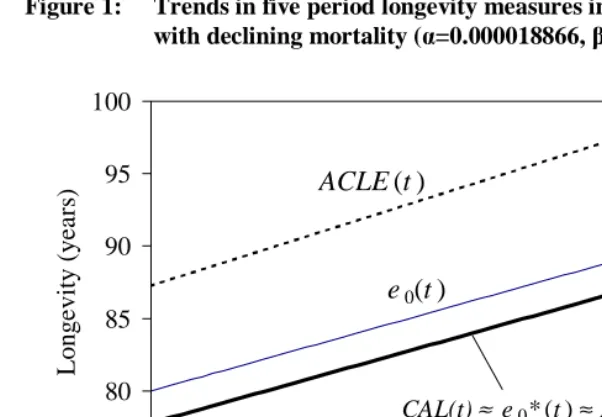
α = 0.00001887 and β = 0.1. With these parameter values e0(t) equals 80.0 years at time t=0. The trend in e0(t) during the 50 year simulation depends on the rate of mortality improvement. With ρ = 0, e0(t)remains constant, with ρ = 0.01 it rises linearly to 85 years and with ρ = 0.02 it rises linearly to 90 years. The simulation results are presented in Table 1. Figure 1 plots values for ρ = 0.02 .

Demographic Research: Volume 13, Article 21

differences arise, but three of the measures are nearly equal to one another throughout the simulation period:

)

(

)

(

*

)

(

t

e

t

LCLE

t

CAL

≈

≈

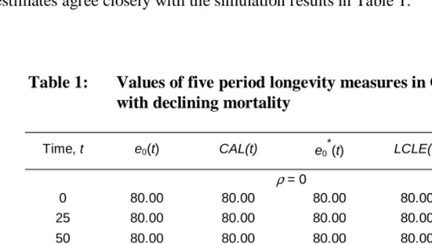
However, e0(t) is higher than these three measures and ACLE(t) is much higher still. The simulations in Table 1 were repeated for different values for α, β with similar results. Lower values of α raised all estimates for all measures by the same amount, but kept the difference between them unchanged. Variations in β also made a difference but results will not be presented here because empirical estimates differ little from 0.1. The effect of changes in values of β as well as ρ can be estimated with an equation obtained by Bongaarts and Feeney (2002). They prove that the difference e0(t) – e0*(t) (called the tempo effect) can be estimated as –1n(1– de0*(t) / dt) / β = –1n(1–ρ / β) / β) if mortality follows a Gompertz pattern with a constant rate of change in the force of mortality. According to this equation the difference between e0(t) and e0*(t) equals 1.05 years when ρ = 0.01 and 2.23 years when ρ = 0.02 (assuming β = 0.1). These analytic estimates agree closely with the simulation results in Table 1.

Table 1: Values of five period longevity measures in Gompertz model with declining mortality

Time, t e0(t) CAL(t) e0

*

(t) LCLE(t) ACLE(t)

ρ = 0

0 80.00 80.00 80.00 80.00 80.00 25 80.00 80.00 80.00 80.00 80.00 50 80.00 80.00 80.00 80.00 80.00

ρ = 0.01

0 80.00 78.96 78.96 78.97 83.23 25 82.50 81.46 81.45 81.46 85.87 50 85.00 83.95 83.95 83.96 88.50

ρ = 0.02

Figure 1: Trends in five period longevity measures in a Gompertz model with declining mortality (α=0.000018866, β =0.1, ρ=0.02)

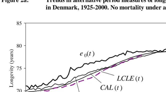
Figures 2a, b, c plot estimates of four of the five period measures of longevity for females in Denmark, England and Wales, and Sweden from 1925-2000. Each measure is calculated with µ(a,t) = 0 for a<30 to insure that the shifting assumption holds approximately. ACLE(t) is not included because its estimation requires projections of future mortality for more than a century. The results are consistent with the simulations: conventional life expectancy is higher than the other measures and CAL(t) ≈ e0*(t) ≈

LCLE (t) in recent decades. 75

80 85 90 95 100

0 10 20 30 40 50

Time (years)

Longe

vity (

y

e

a

rs)

Tempo effect

ACLE (t )

e

(t )

Demographic Research: Volume 13, Article 21

Figure 2a: Trends in alternative period measures of longevity for females in Denmark, 1925-2000. No mortality under age 30.

65 70 75 80 85

1925 1950 1975 2000

Longevity (years)

_{CAL (t )}

LCLE (t )

e

(t )

e

*(t )

Figure 2b: Trends in alternative period measures of longevity for females in England and Wales, 1925-2000. No mortality under age 30.

65 70 75 80 85

1925 1950 1975 2000

L

onge

vit

y

(

y

e

a

rs

)

e

(t )

CAL (t )

e

*

(t )

Figure 2c: Trends in alternative period measures of longevity for females in Sweden, 1925-2000. No mortality under age 30.

65 70 75 80 85

1925 1950 1975 2000

Longevity (years)

e

(t )

CAL (t )

LCLE (t )

e

*(t )

4. Discussion

A detailed discussion of the alternative longevity measures and their strength and weaknesses is beyond the scope of this descriptive note, and only brief comments on the most noteworthy findings will be provided.

First, in the simulations, three of the period longevity indicators CAL(t), e0*(t) and

LCLE (t) are virtually identical to one another. This finding is consistent with the analytic results by Bongaarts and Feeney (2003) who prove that CAL(t) = e0*(t) in populations in which the shifting assumption holds. As noted, pc(a,t – a) is assumed to

Demographic Research: Volume 13, Article 21

changes in CAL(t) are constant). This result is also consistent with the analysis of cohort and period tempo of fertility by Ryder (1980).

Second, the conventional life expectancy at birth e0(t) is substantially higher than three other period measures CAL(t), e0*(t) and LCLE(t). The difference between e0(t) and e0*(t) is constant throughout the simulation but varies with the rate of improvement in mortality: it equals 2.2 years with ρ = 0.02, 1.05 years with ρ = 0.01 and 0 when ρ = 0. These findings are consistent with the mortality tempo effect described by Bongaarts and Feeney (2002, 2003, 2004).

Third, the weighted average cohort life expectancy ACLE(t) is much higher than the other four indicators. This difference is not surprising since the weights applied to the life expectancies of cohorts alive at time t are highest for the youngest (i.e. most recent) cohorts. As a consequence, this measure is heavily influenced by the mortality that young cohorts will experience in the future. This is confirmed by Schoen and Romo (2004) who conclude that ACLE is roughly the arithmetic mean of the period life expectancy at time t and the cohort life expectancy of the cohort born in year t.

The empirical results for females in Denmark, Sweden, and England in Figure 2 are similar to the simulation findings for recent decades i.e., since approximately the 1970s. However, in earlier decades, differences between CAL(t), e0*(t) and LCLE(t), while still small, are no longer negligible. The probable reason for the modest divergence between CAL(t) and e0*(t) before ca.1970 is that the shifting assumption is then less accurate. The reason for the appearance of a small but significant divergence between CAL(t) and LCLE(t) in the earlier period is presumably that the assumption of linear change in CAL(t) is more accurate later than earlier in the last century.

5. Conclusion

6. Acknowledgements

Demographic Research: Volume 13, Article 21

References

Bongaarts, John, and Griffith Feeney. 2002. “How long do we live?” Population and Development Review 28(1): 13-29.

Bongaarts, John, and Griffith Feeney. 2003. “Estimating mean lifetime,” Proceedings of the National Academy of Sciences. 100 (23): 13127-13133.

Bongaarts, John and Griffith Feeney. 2005. “The quantum and tempo of life cycle events,” Policy Research Division Working Paper No. 207. New York City: Population Council.

Brouard, N. 1986. “Structure, et dynamique des populations. La pyramide des années a vivre, aspects nationaux et exemples régionaux,” Espaces, Populations, Sociétés.(2) :14-5, 157-68.

Goldstein, Josh. 2005. “Found in translation? A cohort perspective on tempo-adjusted life expectancy,” Forthcoming, Demographic Research, http://www.demographic-research.org

Guillot Michel. 2003. “The sectional average length of life (CAL): A cross-sectional mortality measure that reflects the experience of cohorts,” Population Studies. 57(1):41-54.

Preston, Samuel H., Patrick Heuveline, and Michel Guillot. 2001. Demography: Measuring and Modeling Population Processes. Malden, MA: Blackwell.

Rodriguez, German. 2005. “Demographic Translation and Tempo Effects: An Accelerated Failure Time Perspective,” Forthcoming, Demographic Research, http://www.demographic-research.org

Ryder, Norman B. 1980. “Components of temporal variations in American fertility,” in R.W. Hiorns (ed.), Demographic Patterns in Developed Societies, London: Taylor & Francis, pp. 15-54.

Schoen, Robert and Vladimir Canudas-Romo. 2005. “Changing mortality and average cohort life expectancy,” Demographic Research: 13-5. pp. 117 - 142

Schoen, Robert, Stefan H. Jonsson and Paula Tufis. 2004. “A population with continually declining mortality,” paper presented at the PAA 2004, Boston.

Vaupel, James W. 1986. “How change in age-specific mortality rates affect life expectancy,” Population Studies 40: 147-157.