The dynamics of the impact and coalescence of droplets on a solid surface

The dynamics of the impact and coalescence of droplets on a solid surface

J. R. Castrej´on-Pita∗1, E. S. Betton1, K. J. Kubiak2, M. C. T. Wilson2, and I. M. Hutchings1

1_{Institute for Manufacturing, University of Cambridge,}

17 Charles Babbage Road, Cambridge, CB3 0FS, United Kingdom. and

2

School of Mechanical Engineering, University of Leeds, Leeds, LS2 9JT, United Kingdom

A simple experimental setup to study the impact and coalescence of deposited droplets is de-scribed. Droplet impact and coalescence have been investigated by high speed particle image ve-locimetry. Velocity fields near the liquid-substrate interface have been observed for the impact and coalescence of 2.4 mm diameter droplets of glycerol/water striking a flat transparent substrate in air. The experimental arrangement images the internal flow in the droplets from below the substrate with a high-speed camera and continuous laser illumination. Experimental results are in the form of digital images that are processed by particle image velocimetry and image processing algorithms to obtain velocity fields, droplet geometries and contact line positions. Experimental results are compared with numerical simulations by the lattice Boltzmann method.

Keywords: Droplets, Velocimetry, Coalescence, Lattice Boltzmann.

PACS numbers: 47.55.db (Drop and bubble formation) and 47.80.Jk (Flow visualization and imaging)

I. INTRODUCTION

The coalescence of droplets on a solid surface is a phe-nomenon with applications in the mixing of reagents in microfluidic systems, biological materials and the print-ing of electronic components. The study of the impact and coalescence of droplets is also important to the inkjet industry as it can strongly influence the quality of print-ing [1–3]. Droplet coalescence occurs throughout nature and also in industrial applications, from rain drop forma-tion to rapid prototyping and sintering. With the inkjet industry expanding into new areas of manufacturing, the accuracy of drop deposition is becoming paramount. For applications such as printed circuit boards or depositing biological materials, the understanding of both the in-ternal and the free surface dynamics is essential to the functionality of the final product. Similarly in the mixing of two substances in microfluidics, the rate and extent of the flow must be controlled.

Several investigations have been carried out to study the dynamics of coalescence of two effectively sessile liq-uid drops. In these experiments, a first, stationary drop is placed on to a substrate and a second drop is caused to grow next to it by feeding fluid through a small hole in the substrate until the edge of the second drop contacts the first and coalescence takes place, [1] and [4]. This process can be analysed by treating it as the coalescence of two sessile drops as the second drop is usually expanded very slowly. In such experiments, the rapid neck growth at the point of connection between the two drops is usually observed from above [5] and/or from the side [4]. So far, these studies have shown that the expansion of the neck is driven by surface tension and is opposed by inertial or viscous forces. In particular, it has been demonstrated that the diameter of the meniscus between the two coa-lescing drops grows in time following a power law. This behavior has been found in the coalescence of mercury droplets, in the coalescence of thin viscous drops

spread-ing by surface tension and in the early stages of spreadspread-ing of both viscous and inviscid fluids, [5–8]. These investi-gations have been focused on externally measured prop-erties such as contact angles, composite diameters and droplet radii, and not on studying the dynamics of the flows within the droplets.

Some previous experimental investigations have been reported which visualized the internal motion in droplets. The internal flow within evaporating drops deposited on a surface has been visualized to demonstrate the exis-tence of symmetric circulation flows which either ascend or descend at the axis of symmetry depending on the mo-tion of the contact line, [3]. Additionally, experiments on the coalescence of two differently coloured droplets have identified the time scales on which the mixing of fluid oc-curs, [1]. Quantitative measurement techniques, such as particle image velocimetry (PIV), on sessile or coalesc-ing droplets encounter several limitations, the most im-portant being the optical distortion effects produced by the differences of refractive indexes between the droplet fluid, the substrate material and the medium by which the fluid is surrounded (commonly air), [9]. Experiments within index-matched liquids have been conducted using, conventional, dual-field and tomographic PIV systems. These experiments have given an accurate insight into the internal flow in colliding and coalescing drops, [10–

12]. Apart from these investigations, little quantitative experimental work has been carried out on the internal flow in drops during impact and coalescence in air.

Coalescence of two static droplets can be divided into three stages. During the initial stage, the droplet edges make contact and quickly form a thin liquid bridge be-tween the two drops, which then increases in width fol-lowing a temporal power law, [1]. During this stage the contact line away from the neck does not move. After this, in the intermediate stage, the neck relaxes; the con-tact line surrounding the droplets begins to move, and the curvature of the drop surface above the initial contact point changes from concave to convex. The final stage

The following article appeared in Biomicrofluidics 5, 014112 (2011)

and may be found athttp://link.aip.org/link/?bmf/5/014112 [email protected]

occurs as the combined drop relaxes towards a spherical cap, the minimum surface energy configuration. There is minimal movement of the contact line during this phase, and pinning of the contact line affects the final footprint of the combined droplet.

This paper presents a novel application of particle im-age velocimetry to the impact and coalescence of a falling droplet and a sessile droplet. The experimental setup is simple and can be applied to systems with non-matching refractive index. Briefly, these experiments consisted of impacting droplets on to a transparent substrate in or-der to observe the internal dynamics through and from below the substrate. In this way, the differences of re-fractive index do not distort the view, no reconstruc-tion algorithms are required and a clear visualizareconstruc-tion can be achieved in a two-phase system (air/liquid). In addition, this work combined shadowgraph imaging on a side-view plane with digital image analysis to extract the traditional geometric properties of the coalescence phenomenon such as dynamic contact angles, composite diameters and neck height and width. Droplets 2.4 mm in initial diameter with Newtonian properties were used in these experiments. Experiments were carried out vary-ing the sideways separation between the sessile and the impacting droplet from the axisymmetric drop on drop case up to the point (≈4.3 mm) of no coalescence. The experimental results are compared with numerical simu-lations based on the lattice Boltzmann method.

A. Experimental method

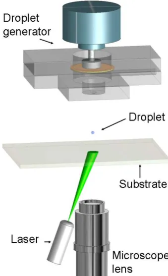
A schematic view of the experimental setup is shown in Fig. 1. As mentioned above, the aim of these exper-iments was to study the internal flow and the dynamics of droplets during deposition and coalescence. The ex-periments consisted of depositing a droplet adjacent to a sessile droplet resting on a transparent substrate. Two imaging arrangements were used: a method to visualize the internal flows within the droplets from beneath the substrate, and a shadowgraph system to observe the im-pact and coalescence behavior of the droplets from a side view.

In all experiments, the position, size and speed of the droplets and the impact properties were determined by a droplet generator (a large-scale model of a single-nozzle ink-jet printhead) which has been described elsewhere, [13]. This droplet generator consists of a closed liquid reservoir with a thin membrane on one side and a noz-zle orifice in the opposite wall. The membrane transmits the motion of an electro-mechanical actuator to produce the internal pressure transient which ejects the droplet. The generator is operated in a drop-on-demand mode in which the speed and size of the droplets produced are determined by the waveform sent to the actuator (LDS V201 vibrator). In these experiments, a nozzle 2.2 mm in diameter was used with a Newtonian mixture of glyc-erol and water (85%:15%). Single pressure pulses were

FIG. 1: (Colour online) Schematic view of the experimental arrangement.

applied with the actuator and adjusted to produce the desired ejection speed and size of the droplets. The mea-sured properties of these droplets are shown in Table 1 and were chosen to represent the dynamics of droplets produced by commercially available drop on demand inkjet systems. This was done by quantifying the surface and viscosity forces of a generic system and matching them via the Reynolds (Re) and Weber (We) numbers. These dimensionless numbers are defined as:

Re = ρud

2µ , We = ρu2_d

2σ (1)

whereρis the density,µthe viscosity andσthe surface tension of the fluid,dis the droplet diameter before im-pact, and u is the impact speed. For the system used in these experiments (see Table 1), Re = 16.0 and We = 27.5 which are in the operating range of most commercial inkjet systems.

Droplets were jetted on to a transparent and optically flat PMMA (Perspex, Lucite) sheet, 5 mm thick, placed 65 mm away from the nozzle. The substrate was mounted on a translation stage with a micrometer control to adjust the separation between the coalescing droplets.The liquid was seeded with titanium dioxide (TiO2) particles of ∼

2µm diameter for the PIV visualization.

Density: ρ= 1222.0±2.0 kg/m3

Viscosity: µ= 100.0±0.5 mPa.s

Surface tension: σ= 64.0±0.5 mN/m

Static contact angle: 63.2±0.2 degrees Droplet speed of impact: u= 1.1±0.1 m/s Droplet diameter (in flight): d= 2.38 ±0.03 mm Time between

droplets deposition: 20.0±0.5 s

Separation of droplet centres: 0.00±0.05 mm 0.90±0.05 mm 1.30±0.05 mm 2.00±0.05 mm 3.00±0.05 mm 3.50±0.05 mm 3.80±0.05 mm

Table 1. Fluid and droplet properties.

The PIV technique requires two successive images taken with a short time interval to determine the mo-tion of particles in a flow. In convenmo-tional PIV, the illu-mination and the frame separation are usually provided and controlled by a twin laser system and a specialized camera, [11]. The correct utilization of this technique de-pends on many different variables and, as a consequence, its application is mostly restricted to systems with sym-metrical geometries and to media with matched refractive indexes. In addition, the measurement of the fluid speed is limited by the frame rate, the field of view and the size and resolution of the CCD sensor and the optical sys-tem used for visualization. The measurement volume of a conventional PIV is determined by the field of view of the camera system and the width of the laser beam illu-minating the flow (usually a laser sheet). In contrast, in micro-PIV, the whole fluid volume is illuminated and the depth of the measurement volume is determined by the depth of field of the imaging system, [14]. In this work, an imaging setup consisting of a high speed camera cou-pled to a microscope lens was used for the image acqui-sition; in an analogue of micro-PIV, the optical charac-teristics of the lens determined the measurement volume. As a result, the time between successive images for the PIV analysis was determined and controlled by the frame speed of the high speed camera. The dimensions of the measurement region of this setup are determined by the field of view and the depth of field of the imaging sys-tem and not by the characteristics of the laser beam. A Phantom V7.3 monochrome high speed camera operat-ing at a frame interval of 333.0µs and a exposure time of 331.0µs (3,000 fps option) was used with a Navitar 12x Zoom microscope lens system for the image acquisition. The camera system was pointed upwards to focus on the region of droplet impact on the substrate surface. The microscope zoom lens was set to produce a field of view

of 10 mm×7.5 mm. Under these conditions, the depth of field produced by the optical system was<200µm and a resolution of 80 pixels/mm was achieved.

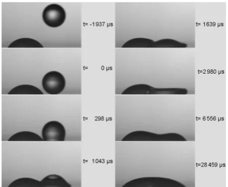
FIG. 2: (Colour online) Examples of images of drop impact and coalescence obtained from the high speed imaging setup

for the case of a droplet separation of 3.00±0.05 mm. The

left-hand images are the original images. The right-hand im-ages are digital negatives which assist the visualization of the contact line position.

The axial position of the camera was adjusted to place the focal region on the substrate plane; as a result the thickness of the measurement volume corresponds to the fluid contained in the first 200 m from the substrate sur-face. The region of droplet impact and coalescence was illuminated with a laser beam 10 mm diameter at the substrate surface, from a CW laser diode with a wave-length of 532 nm and a maximum power of 200 mW, expanded by a 16.5 cm focal length aspheric lens.

The angle of incidence and the position of the laser beam were chosen to minimize reflections. The maximum amplitude region of the beam was centered at the edge of the sessile droplet opposite to the impact point. The laser beam was delivered with an angle of incidence of 27 degrees. For these experiments, the laser was operated at its maximum power, the camera set to its maximum sensitivity and the frame speed and size chosen to be the fastest and largest possible to obtain a clear view of the coalescence process. Examples of the images acquired by this method are shown in Fig. 2.

A second visualization arrangement was used to

The following article appeared in Biomicrofluidics 5, 014112 (2011)

and may be found athttp://link.aip.org/link/?bmf/5/014112 [email protected]

FIG. 3: (Colour online) Examples of images of drop impact

and coalescence obtained by high-speed shadowgraphy. In

these images the droplet offset is 3.00 ±0.05 mm. In both

this series and the one in Fig.2, the time t = 0µs corresponds to the image showing the impacting droplet at the closest

position to the substrate. As a consequence, a systematic

timing error of up to 150µs can exist between this side view

and the bottom view shown in Fig. 2.

serve the impact and coalescence of droplets from a side view, parallel to the substrate plane. For this, the high-speed camera was used with a macro Tamron SP AF90 lens set to its maximum magnification and maximum aperture. For the illumination, a 20×20 cm acrylic op-tical diffuser was placed between the substrate and a 500 W halogen lamp. The camera axis was angled downwards by a few degrees to show the baseline (droplet/substrate interface) clearly. Under these conditions, the high-speed camera was operated at a frame interval of 149.0µs and a exposure time of 2.0µs. The resolution obtained in this setup was 40 pixels/mm, and examples of the recorded images are shown in Fig. 3.

B. Image analysis

The images obtained experimentally with the appa-ratus described above were analyzed digitally to mea-sure the geometrical features of the coalescence pro-cess. Bottom-view images were analyzed to determine the composite droplet length, neck width and left and right droplet radii. Side-view shadowgraph images were studied to establish the neck height and the contact an-gle. A diagram showing these properties is shown in Fig.

4. The Canny edge detection technique (in Matlab soft-ware) was used to find the drop outline in all the images. For the bottom-view, the maximum left and right points were then identified. The image was divided into two parts vertically down the center and the maximum and minimum vertical positions on each side were found. By combining these with the coordinates of the respective

FIG. 4: (Colour online) Diagram showing the quantities de-termined by the image processing. The dotted line indicates the position of the contact line. R1is the radius of the sessile drop, R2 is the radius of the impacting drop, Rx is the neck

width,lis the composite length and Lx is the neck height.

side position, the intersecting chord theorem was used to estimate the radii of the left (R1) and right (R2) drops

individually.

The neck width was found by splitting bottom-view images across the horizontal axis and analyzing the top and bottom sections of the neck. The neck was deter-mined as the point closest to the central axis between the two maxima of the left and right drop peaks. From these coordinates the neck width and position from the left and right edge were found (Rx and l). In a similar

way, side-view images were analyzed to obtain the neck height (Lx).

II. SIMULATION OF DROPLET COALESCENCE BY THE LATTICE

BOLTZMANN METHOD

The droplet coalescence process was also analysed nu-merically using the lattice Boltzmann (LB) method [15]. This mesoscopic approach has the benefit that liquid free surfaces do not require special tracking or reconstruction at each time step; they arise naturally as part of the (liquid-gas) phase separation model, which in this case is the popular Shan-Chen multiphase model [16]. In ad-dition, there is no need to specify the dynamic contact angle as a geometrical constraint at the contact line. In-stead, the surface energy of the solid is effectively spec-ified through a parameter related to the static contact angle via Young’s equation. These features make the method well suited to the simulation of flows involving both large and topological changes in free-surface shape, such as arise in droplet impact and coalescence. The LB

method is also algorithmically much simpler than other diffuse-interface methods.

The ‘lattice’ in the LB method represents a discreti-sation of both 3D space and molecular velocity. Each node in the lattice has a set of vectors,~ea(a= 0, . . . ,18),

given by the displacements from the node to its 18 nearest neighbours plus the zero vector. The vectors~earepresent

19 molecular velocities, and each of these has associated with it a probability distribution function, fa. The

val-ues of fa across the whole lattice evolve in time

accord-ing to a simple two-step process repeated at each time step: (i) thefa at each lattice node relax towards a local

Maxwellian distribution, and (ii) eachfa ‘streams’ along

its associated vector to the neighbouring node. Thus step (i) represents molecular collision and step (ii) molecular motion.

Using a simple single relaxation time,τ, for all thefa,

the process can be written as

fa(~x+~ea, t+ ∆t) =fa(~x, t)−

[fa(~x, t)−faeq(~x, t)]

τ (2)

where the local Maxwellian equilibrium distribution is given by:

f_aeq(~x, t) =waρ

1 + 3~ea·~u c2 +

9 2

(~ea·~u)2

c4 −

3 2 ~ u2 c2

(3)

for a = 0, . . . ,18. Here wa are weights associated with

each vector~ea,~xis the position within the lattice,t the

time, ∆t the time step, and c the lattice speed, whileρ and~uare repectively the macroscopic density and veloc-ity calculated as follows:

ρ(~x, t) =

18 X

a=0

fa(~x, t) (4)

~ u(~x, t) =

18 X

a=0

~eafa(~x, t)/ρ(~x, t) (5)

For multiphase capability, the Shan-Chen model [16] introduces an interaction potential between neighboring lattice nodes, which can be expressed as:

F(~x, t) =−Gψ(~x, t)

18 X

a=0

waψ(~x+~ea, t)~ea (6)

whereFis fluid-fluid interaction force,Gis an interaction strength parameter (negative for particle attraction), and ψis a potential function that depends on density:

ψ(ρ) =ρ0[1−exp(−ρ/ρ0)] (7)

whereρ0= 1. This model produces a non-ideal equation

of state that supports the coexistence of a heavy phase of densityρh and a light phase of densityρl.

In order to simulate a droplet impacting onto a solid surface, a surface wetting model must also be introduced. Here this is achieved by specifying the fluid density on

the solid surface via a ‘surface affinity’ parameter [17] defined in the range 0 to 1 by:

η=ρw−ρl ρh−ρl

(8)

where ρw is the density at the wall. Specifying η and

using the calculatedρwresults in an equilibrium contact

angle between 0◦ (η = 1) and 180◦(η= 0). In this study the choiceη = 0.4 is used to give a static contact angle ofθs= 63◦. Owing to the diffuse nature of the interface,

only this static contact angle is required as an input; the dynamic contact angle, which varies around the con-tact line, emerges as a result of the simulation. In this kind of model, the contact line moves via an evaporation-condensation mechanism.

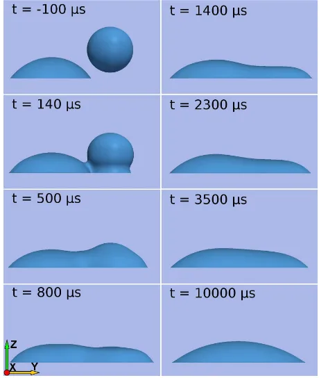
FIG. 5: (Colour online) Lattice Boltzmann simulation of

droplet impact and coalescence corresponding to that in Fig. 3.

The above approach is sufficient to simulate the wetta-bility of a perfectly smooth surface. However, the prop-erties of the surface can have a large influence on droplet deposition, spreading and coalescence. Owing to contact angle hysteresis, in the experiments (see below) only a small retraction of the contact line can be observed and the final footprint of the droplets after coalescence covers almost the same surface that was wetted during impact. For improved simulation of this phenomenon, a wetting model taking into account contact angle hysteresis and fluid adhesion on the solid surface is required. The sur-face affinity parameter (8) is initially set to correspond to the advancing contact angleθa = 85◦ measured from

the experiments. Once the surface at a given location is

The following article appeared in Biomicrofluidics 5, 014112 (2011)

and may be found athttp://link.aip.org/link/?bmf/5/014112 [email protected]

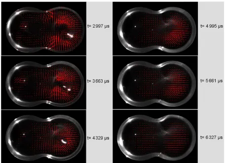
FIG. 6: (Colour online) Velocity fields for the coalescence of two glycerol/water droplets. The droplet on the right had impacted the substrate at a time t = 0µs; the droplet on the left had been deposited 10 s earlier and can be considered sessile. The droplet separation is of 3.00±0.05 mm. The velocity vectors around the laser reflections are spurious and should be ignored.

wetted, i.e. when for the first node above the bottom wall (z+ 1):

ρ(x, y, z+ 1)≥ρl+Hr(ρh−ρl), (9)

the local static contact angle changes and the surface affinity at relevant nodes is changed to match the reced-ing contact angleθr= 54◦, i.e.η=f(θr). HereHr= 0.9

is a threshold parameter governing when the change will be applied. On the other hand, when the contact line starts to retract and the surface is dewetted, i.e. when

ρ(x, y, z+ 1)≤ρl+Ha(ρh−ρl), , (10)

the surface at the given location starts to recover its ini-tial properties, i.e. the local static contact angle reverts to θa over a timeTe, which corresponds to the physical

time needed for evaporation of liquid molecules from the dewetted surface. This means that the local value of the static angle will gradually change fromθrto θa over the

time periodTe. In this case linear interpolation is used.

Henceη =f(θa, Te) in this case. The threshold

parame-ter Ha (= 0.1) again controls the surface conditions

un-der which this change is initiated. The value of this and

the other wetting model parameters have been chosen by comparing the simulation of a single droplet deposition with experimental results in order to obtain a similar fi-nal footprint. Such a wetting model gives more flexibility to define fluid-solid interactions and improve the ability to capture the effect of contact angle hysteresis in lat-tice Boltzmann simulations. Fig.5shows a visualisation of the lattice Boltzmann simulation corresponding to the experimental conditions in Fig.3.

The parameters used for the LB simulations are deter-mined by matching the experimental conditions as closely as possible. The parameter Gcontrols both the surface tension and the density ratio between the liquid droplet and the surrounding fluid. It was set atG=−4.5, giv-ing dimensionless densitiesρh = 1.493,ρl= 0.253. The

initial droplet diameter was 40 lattice nodes, which in physical units for d= 2.38mm gives the lattice spacing between nodes as dx = 5.95·10−5_{m. The relaxation}

times for the two phases were chosen as τh = 1.0 and

τl = 0.9. Choosing different relaxation times for the

heavy (ρh) and light (ρl) fluids allows the viscosity

ra-tio to be changed. The timestep,dt, is a free parameter which is usually used in combination with the relaxation times to set the fluid kinematic viscosity. In this case the

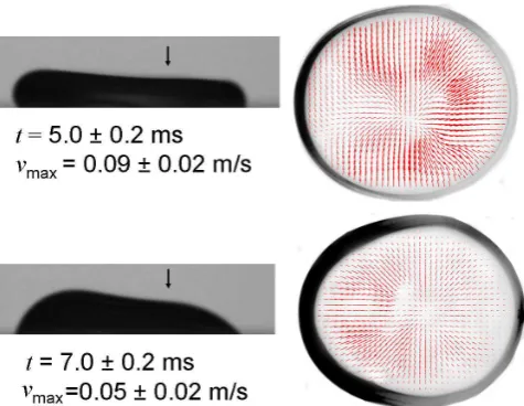
FIG. 7: (Colour online) Velocity fields for the coalescence of two glycerol/water droplets. The center to center separation between the sessile (left) and the impacting (right) droplet is

1.30±0.03 mm. On the left, a shadowgraph image shows the

side-view of the coalescence at the same time. The reported maximum speed corresponds to the magnitude of the longest vector on the field. Note that the downward vertical arrow in the shadowgraphs indicates the center of the impacting droplet.

resulting value was dt = 3.0·10−6_{s. The acceleration}

due to gravity in lattice Boltzmann units was 1.48·10−6_.

Because of model limitations, the numerical density ratio between the fluids is about 6, however keeping the vis-cosity ratio similar to the physical value it is possible to recover the fluid dynamics of the impact, spreading and relaxation phases.

To initialise the impact and coalescence simulations, a single sessile droplet was first simulated and allowed to come to equilibrium. A second droplet was then added to the computational domain a short distance above the sessile droplet. This impacting droplet was given a speed and offset corresponding to the impact speed and offset in the experiments.

III. RESULTS

A. Experimental

Experiments were carried out varying the separation between the sessile and the impacting droplet from the axisymmetric drop on drop case up to the point (ap-prox 4.3 mm) of no coalescence. High speed bottom-view images were analyzed by using two particle image velocimetry codes, URAPIV and MatPIV, with similar results, [18, 19]. Consecutive high speed pictures were analyzed to detect the motion of the seeded particles to obtain the internal velocity fields. As previously men-tioned, the correct application of PIV analysis is condi-tioned to several variables including the particle

displace-FIG. 8: (Colour online) Velocity fields for the coalescence of

two droplets whose centers are separated by 2.00±0.03 mm.

On the left, a shadowgraph image shows the side-view of the coalescence at the same time. The reported maximum speed corresponds to the magnitude of the longest vector on the field.

FIG. 9: (Colour online) Velocity fields for the coalescence of

two droplets whose centers are separated by 3.80±0.03 mm.

On the left, a shadowgraph image shows a side-view of the coalescence stage at the same time. The reported maximum speed corresponds to the magnitude of the longest vector on the field.

ment criterion. In these experiments, PIV analyses were only applied to image pairs showing a maximum particle displacement of less than 10 % of the size of the interroga-tion area (64×64 pixels). As a result, appropriate PIV analyses were performed using consecutive images taken 3 ms after impact. This time corresponds to the region after maximum spreading, a phase usually described as the relaxation regime, [20]. Velocimetry studies at earlier times were restricted by the frame speed of the camera which was limited by the light conditions and its sensi-tivity. Experimental PIV results are shown in Figs. 6,7,

8and9.

The velocity vectors surrounding the center of the re-cently deposited droplet suggest the existence of a dis-tinctive flow circulation pattern in which fluid rises near the centre of the impacting droplet. This is consistent with the growth in free-surface height in that region

The following article appeared in Biomicrofluidics 5, 014112 (2011)

and may be found athttp://link.aip.org/link/?bmf/5/014112 [email protected]

FIG. 10: (Colour online) Side-view shadowgraph imaging of the coalescence of an impacting and a sessile droplet. The droplet separation corresponds to the droplet center to center distance.

served from the shadowgraph images. The position of the upward flow moves towards the center of the com-posite drop at a rate dependent on the separation of the droplets as can be observed in Figs. 6to9.

It is interesting to observe in Fig. 8 that, at the left-hand edge of the upper PIV image, the flow is to the left, towards the contact line. This indicates that the fluid in that part of the sessile droplet is still being pushed to the left by the wave that travels right to left after the impacting droplet lands on the sessile one. This is con-sistent with observations of the left-hand contact angles in the two shadowgraphs presented in Fig.8and suggests a flow up the free surface at that stage.

In Figs.7and8, the offset between the droplet centers is such that there is a substantial interaction between the two droplets, with the flow induced in the sessile droplet being similar in magnitude to that in the impact-ing droplet. Fig.9shows images for a much larger droplet offset, approaching the limit of separation at which co-alescence is still possible. Here, as is to be expected, the impacting droplet behaves much more like an iso-lated droplet, and the flow induced in the sessile droplet is very weak.

For the experiments shown here it can be observed that the different stages of coalescence depend on the distance between the droplets. Side-views of the coalescence of an impacting droplet on a sessile one at different droplet separations are shown in Fig. 10. When there is no offset between the centers of the two droplets, the result is the expected axisymmetric impact and spreading, and the contact area of the combined droplet remains circular. When the droplet separation is increased to 0.9 mm, it can be observed that, prior to impact, the right edge of the impacting drop still lies inside the right edge of the

sessile drop. This implies that when the drop impacts it lands completely on pre-wetted substrate. Though the evolution of the free surface is no longer axisymmetric, and the contact line at the left edge of the sessile droplet remains pinned, this impact results in the same circular footprint shape as in the axisymmetric impact.

For larger offsets (e.g. 2.00 mm) the impacting drop lands partially on pre-wetted substrate and partially on dry substrate. Once the droplet offset is greater than the radius of the sessile droplet plus the radius of the droplet in flight (droplet separations> R1+d/2) the impacting

drop lands entirely on dry substrate and therefore im-pacts and spreads before coalescence occurs. After land-ing, the impacting drop spreads and then merges into the sessile droplet making the coalescence more like the one observed between two sessile drops (though differences still exist as explained below).

For a single drop the spreading process is divided into the impact and wetting stages. The impact stage consists of the kinematic phase, spreading phase and relaxation phase. For long drop separations, the initial stage of co-alescence between a sessile drop and an impacting drop can be divided into the same three phases. The side view images in Fig. 3 show the drop impact and spreading. The kinematic stage occurs for the first few hundred mi-croseconds as the fluid in the impacting drop is moving vertically downwards. Beyond this point, fluid begins to spread horizontally. This corresponds to the spreading phase of impact. This is when coalescence between the two drops starts. The fluid spreads outwards and the drop height of the impacting drop decreases, forming a flattened disc shape corresponding to a maximum diam-eter; this occurs after approximately 3 ms. As the height of the impacting drop decreases below that of the sessile

drop it can be assumed that the inertia causing the drop spreading is greater than the hydrostatic forces of the bulk fluid above. During the relaxation phase of spread-ing, or the intermediate stage of coalescence, the height of the impacting drop increases and the surface curvature decreases. After around 30 ms the drop reaches the final stage of coalescence and starts to relax into a spherical cap shape. The drop does not reach a spherical cap shape due to hysteresis of the contact angle causing pinning.

FIG. 11: (Colour online) Temporal evolution of the measured droplet and neck features determined from image processing for a system with a droplet separation of 3.00 mm.

The external dynamics of the impact and coalescence process, for a system with a droplet separation of 3.00 mm, are quantified in Fig.11, which shows the measured droplet radii (defined in Fig.4), and the width and height of the growing ‘neck’ between them. The radius of the pre-deposited sessile droplet is remarkably unaffected by the impact of the second droplet. The radius of the im-pacting droplet grows very rapidly and expands beyond that of the sessile droplet as it spreads into its flattened disc, then it enters the retraction and much slower relax-ation stage captured in the PIV results of Fig.6.

For systems where the separation between droplets is > R1 +d/2 the growth of the neck height is

partic-FIG. 12: (Colour online) Temporal evolution of the composite length (l) for various droplet separations.

ularly telling when considering the differences between the impact-driven coalescence considered here and the capillary-driven coalescence of two static droplets. As the impacting droplet spreads, it quickly pushes into the sessile droplet and swiftly closes the gap between them. The neck height therefore increases very rapidly in this stage, until it becomes commensurate with the height of the disc formed when the impacting droplet is at its maximum extent. At this stage it is difficult to define a clear ‘neck’ in the side views (Figs.3and5), and the neck height profile shows a plateau corresponding to the height of the flattened impacting droplet. However, the flat-tened droplet then begins to recover; its height increases, and a distinct neck once again forms, which grows much more slowly. From this point the development is similar to the static coalescence case.

Fig. 12 shows the composite spread length, l, mea-sured during impact and coalescence for different off-sets between the centers of the sessile and impacting drops. When comparing the change in composite length for the 0 mm offset and 0.9 mm there is no variation between the two cases. As remarked above, both these cases produce a combined droplet with the same circu-lar contact footprint. There is an intriguing difference in the behaviour for the intermediate offsets, 3.00 mm and 3.50 mm: the composite droplet length shrinks slowly in a second phase of adjustment of the composite droplet. This is attributed to a slow expansion of the neck in these intermediate cases, but it is evidently a non-trivial effect that requires further exploration. The footprints of the composite droplets at 0.6 s after impact are shown in Fig.

13. These highlight the importance of contact line pin-ning in determipin-ning the shape of the composite droplets.

The following article appeared in Biomicrofluidics 5, 014112 (2011)

and may be found athttp://link.aip.org/link/?bmf/5/014112 [email protected]

FIG. 13: (Colour online) Footprints for various droplet spac-ings. These images were taken 0.6 s after the first contact of the droplets.

B. Computational

It has been observed before [21] that diffuse-interface models of wetting, such as the lattice Boltzmann method used here, have a tendency to overpredict the speed at which wetting occurs because, for computational ef-ficiency, the liquid-gas interface thickness is generally larger than the true thickness. This effect is also seen in the simulations presented here, which show the coales-cence process happening more quickly than in the exper-iments. However, it is interesting to check the qualitative behavior of the model against the experimental data.

The simulation predictions of the droplet radii and neck growth are given in Fig. 14for different offsets be-tween the droplet centers. Despite over-predicting the rate at which the changes occur, the simulation captures well the essential features such as the spreading of the impacting droplet to its maximum extent, and subse-quent recoil. As observed experimentally, the simulations predict very similar droplet radii when the offset of the droplets is zero or 0.9 mm, and when the offset is 3.00 mm the radii of the sessile and impacting droplets are essen-tially equal (as seen in Fig. 11). These results are also consistent with the radii of the two droplets seen in the footprints shown in Fig.13, which show that for large off-sets, the radius of the impacting droplet ends up smaller than that of the sessile droplet.

The growth of the neck height again shows the differ-ent behaviour at differdiffer-ent stages: the very rapid initial in-crease in height as the gap between the droplets is closed, and the later, slower relaxation. However, the simulation overpredicts the extent to which the impacting droplet merges with the sessile one in the initial impact stage (as can be seen by comparing Fig.5with Fig.3). Hence there is actually an initial peak in the neck height plot (Fig.14), followed by a reduction in neck height as the impacting droplet flattens. Again, the ‘neck’ is not dis-tinct at this stage. Another cause for a slight discrepancy between the simulation and experiment is that in the

sim-0 5 10 15 20

time [ms] 0.0

0.5 1.0 1.5 2.0 2.5 3.0

Droplet radii [mm]

Sessile droplet 0.0 mm 0.9 mm 2.0 mm 3.0 mm 3.5 mm 3.8 mm 4.2 mm

Droplet separation - (lattice Boltzmann)

0 5 10 15 20

time [ms] 0.0

1.0 2.0 3.0 4.0 5.0

Neck width [mm]

0.9 mm 2.0 mm 3.0 mm 3.5 mm 3.8 mm 4.2 mm

Droplet separation (lattice Boltzmann)

0 5 10 15 20

time [ms] 0.0

0.2 0.4 0.6 0.8 1.0 1.2 1.4 1.6 1.8 2.0

Neck height [mm]

0.9 mm 2.0 mm 3.0 mm 3.5 mm 3.8 mm 4.2 mm

Droplet separation (lattice Boltzmann)

FIG. 14: (Colour online) Evolution of the droplet and neck features calculated from the lattice Boltzmann simulation.

ulation the neck height is calculated based on the local minimum in the free surface height measured along the centreline. Hence any concavity on the surface would produce a lower value of the neck height since in the experimental side view, it is impossible to see past the higher, outer part of the droplet.

Note that the neck growth curves shown in Fig. 14

for an offset of 4.2 mm do not exhibit the complex be-haviour seen in the other cases. This offset is very close to the limit of separation (≈4.3 mm) that still allows

FIG. 15: (Colour online) Velocity fields calculated from the Lattice Boltzmann simulation of the coalescence of two droplets.

The droplet on the right had impacted the substrate at a time = 0µs, the droplet on the left was deposited in a previous

simulation and is considered sessile; the droplet separation is 3.00 mm. Note that for clarity the velocity vectors are shown at different scales in the two columns. The longest vector in the left-hand column corresponds to a speed of 1.5 m s−1; the longest vector in the right-hand column represents 0.05 m s−1

.

lescence to occur. In this scenario, the impacting droplet is almost at full stretch when it makes contact with the sessile droplet. It is therefore effectively stationary at this point, and coalescence proceeds in a manner very simi-lar to that seen in the coalescence of two sessile droplets [1,4].

Fig. 15 shows the droplet impact simulation viewed from below the substrate, mimicking the arrangement of the experimental PIV system, and showing the calcu-lated velocity vectors. The offset of the droplet centers was 3.00 mm. The images in the left-hand column of the figure show the spreading stage of the droplet deposition, while those on the right show the retraction. Focusing on the right-hand column, these show good agreement with the generic features of the experimental PIV results of Fig. 6: the flow is focused towards a point on the cen-treline between the neck and the center of the impacting droplet. As in the experiments, the flow is mainly from the right, consistent with the recoil of the droplet seen in Fig. 3. The longest vector in the right-hand column corresponds to a speed of 0.05 m s−1_{, which is consistent}

with the experimental PIV presented in Figs.7–9. The footprint of the combined drop does not show as pro-nounced a ‘peanut’ shape as in the experiments, but with the inclusion of contact angle hysteresis in the model it does retain an elongated shape rather than relaxing to the circular footprint that would result if no hysteresis were present.

To give an indication of the speed of flow in the ear-lier stages of the impact and coalescence, the left-hand column of Fig. 15shows the expansion stage of the im-pacting drop. It is important to note the difference in scale of the velocity vectors in the two columns, which is essential to allow the flow structure to be seen. In the left-hand column, the length of the longest vector repre-sents a speed of 1.5 m s−1_{. This indicates that the fluid}

velocities that arise in the initial stage of the impact and coalescence process are some 30 times greater than those arising in the relaxation stage. This highlights the chal-lenge in visualizing the internal dynamics of the droplets in the earlier stages using PIV. The simulation results also indicate that the pre-deposited droplet is essentially

The following article appeared in Biomicrofluidics 5, 014112 (2011)

and may be found athttp://link.aip.org/link/?bmf/5/014112 [email protected]

inert in the initial coalescence stage for this value of the droplet offset.

0 5 10 15 20

2 3 4 5 6 7 8 0.0mm 0.9mm 2.0mm 3.0mm 3.5mm 3.8mm l , co m p o si t e l e n g t h [ m m ] time [ms] Droplet Separation (lattice Boltzmann) Sessile droplet diameter

FIG. 16: (Colour online) Evolution of composite droplet

length calculated from the lattice Boltzmann simulation.

Fig.16shows computational predictions of the length of the composite droplet as a function of time, for differ-ent values of the droplet separation. This is the equiva-lent of Fig.12, but over a shorter time period. As in the experiments,l is essentially unchanged when the droplet offset is increased from zero to 0.9 mm, and the predicted value compares very well with the experiments in these cases. Agreement is less good at higher droplet offsets, for which the simulations overpredict the degree of contrac-tion of the composite droplet. This is attributed to the simplicity of the model for contact angle hysteresis and the complexity of the contact line behaviour in practice, which leads to the non-trivial contact line shapes seen in Fig.13. It should be pointed out, however, that with no hysteresis included, the ultimate composite length pre-dicted by the simulations would be the same for every case, because there would be no mechanism to prevent the contact line from contracting to a circle.

IV. CONCLUSIONS

An experimental configuration has been presented that allows the visualization of the internal dynamics and sur-face motion of drops impacting and coalescing on a trans-parent substrate. In particular, the coalescence of a ses-sile droplet with a second droplet impacting on or ad-jacent to it has been explored, and a parametric study conducted to reveal the effect of the sideways separation of the droplets. Particle image velocimetry has been used to obtain the internal velocity field within the coalescing droplets during the recoil of the impacting droplet.

The velocity fields exhibit a locally radial flow inwards, indicating a region of upward fluid motion consistent with the elevation of the free surface as the impacting droplet

recoils. For small offsets between the droplet centers, the flow in each droplet is of a similar magnitude; as the sep-aration increases, the sessile droplet becomes essentially inert, with only a weak flow induced by the impact.

Side-view shadowgraph pictures of the same experi-ments were analyzed to determine the geometrical char-acteristics of the coalescence process. For small droplet separations, the impacting droplet lands entirely on pre-wetted substrate, and the spreading process is similar to the axisymmetric case, leading to a circular final foot-print. For larger separations, the impacting droplet lands on dry substrate, then spreads into the sessile droplet. In such cases, the growth of the neck height, in particular, highlights the difference between this impact-driven coa-lescence and the coacoa-lescence of two static droplets. The neck height initially increases more rapidly in the impact-driven case, as the gap between the droplets is closed by the rapid spreading of the impacting droplet. The neck then becomes difficult to distinguish from the side view, and the height levels off at the height of the fully spread impacting droplet, before becoming more distinct again as the droplet regains its height and coalescence proceeds as in the static droplet case. When the droplet separation is close to the maximum that still results in contact be-tween the droplets, the impacting droplet is fully spread when it meets the sessile droplet and coalescence then proceeds in a very similar way to the case of two static droplets.

The droplet impact and coalescence was also simulated using a lattice Boltzmann method including a model for contact angle hysteresis. The simulations slightly over-predict the speed at which coalescence takes place, but capture the main features of the process. The comparison of the experimental and computational results presented here highlights two important points. First, the quantita-tive differences between the experimental and numerical data demonstrate the need for good experimental visu-alization and quantification of flows, both internally and externally, in order to validate computational methods. Second, the numerical predictions of the fluid velocities that arise in the early stages illustrate the challenges in developing experimental systems capable of analysing the internal dynamics of droplets in the early stages of im-pact and coalescence. Finally, it is remarked that pinning of the contact line has a large influence on the formation and evolution of the neck, and the shape of the final footprint of the composite droplet. This aspect of the flow warrants future investigation, and the droplet coa-lescence system described here is a particularly appealing one for testing models of contact angle hysteresis.

Acknowledgments

This work was supported by the Engineering and Physical Sciences Research Council (UK) and industrial partners in the Innovation in Industrial Inkjet Tech-nology project, EP/H018913/1, and by EPSRC grant EP/F065019/1. ESB wishes to acknowledge support from FFEI Ltd.

[1] M. Sellier and E. Trelluyer, Biomicrofluidics, 3 022412 (2009).

[2] R.E. Saunders, J.E. Gougha and B. Derby,Biomaterials,

29193 (2008).

[3] M. Kaneda,et.al.,Langmuir,249102 (2008).

[4] N. Kapur and P.H. Gaskell, Phys. Rev. E, 75 056315

(2007).

[5] A. Menchaca-Rocha, A. Mart´ınez-D´avalos, R. N´u˜nez, S. Popinet, S. Zaleski,Phys. Rev. E,63046309 (2001). [6] J. Eggers, J.R. Lister, H.A. Stone, J. Fluid Mech., 401

pp. 293-310 (1999).

[7] L. Duchemin, J. Eggers, C. Josserand, J. Fluid Mech.,

487pp. 167-178 (2003).

[8] W.D. Ristenpart, P.M. McCalla, P.V. Roy, H.A. Stone,

Phys. Rev. Lett.,97064501 (2006).

[9] K.H. Kang, S.J. Lee, C.M. Lee and I.S. Kang,Meas. Sci. Technol.,151104 (2004).

[10] C. Verdier and M. Brizard, Rheologica Acta, 41 214

(2002).

[11] C. Ortiz-Due˜nas, J. Kim and E.K. Longmire,Exp. Fluids,

49111 (2010).

[12] J. Kim and and E.K. Longmire, Exp. Fluids, 47 263

(2009).

[13] J.R. Castrej´on-Pita, G.D. Martin, S.D. Hoath and I.M. Hutchings,Rev. Sci. Instrm.,79075108 (2008).

[14] S.A. Hags¨ater, C.H. Westergaard, H. Bruus and J.P. Kut-ter,Exp. Fluids,44211 (2008).

[15] S. Succi,The Lattice Boltzmann Equation for Fluid

Dy-namics and Beyond, Oxford University Press (2001).

[16] X. Shan and H. Chen, Phys. Rev. E, 47 1815–1819

(1993).

[17] D. Iwahara, H. Shinto, M. Miyahara and K. Higashitani,

Langmuir,19(21), 9086 (2003).

[18] Z. Taylor, R. Gurka, A. Liberzon and G. Kropp,

Pro-ceedings of the 61st Annual Meeting of the Division of Fluid Dynamics of the American Physical Society, San Antonio, Texas, November 23-25 (2008).

[19] J. K. Sveen, An Introduction to MatPIV v.1.6.1,

(De-partment of Mathematics, University of Oslo, ISSN 0809-4403, 2004).

[20] W.K. Hsiao, S.D. Hoath, G.D. Martin and I.M. Hutch-ings Journal of Imaging Science and Technology, 35

050304 (2009).

[21] J.M. Yeomans,Physica A,369, 159-184 (2006).