Forward Vertical Integration: The Fixed Proportion Case Revisited

Munich Personal RePEc Archive

Forward Vertical Integration: The

Fixed-Proportion Case Revisited

Bonroy, Olivier and Larue, Bruno

September 2006

Forward Vertical Integration:

The Fixed-Proportion Case Revisited

Olivier Bonroy

Department of Rural Economy and Management Agrocampus Rennes

Center for Research on the Economics of Agri-Food (CREA) Université Laval

[email protected]

and

Bruno Larue

Canada Research Chair in International Agri-Food Trade CREA, Université Laval

[email protected]

September 2006

Abstract: Assuming a fixed-proportion downstream production technology, partial forward

integration by an upstream monopolist may be observed whether the monopolist is advantaged or disadvantaged cost-wise relative to fringe firms in the downstream market. Integration need not induce cost predation and the fringe firms’ margin may even increase. The output price falls and welfare unambiguously rises.

Keywords: Vertical integration, cost predation, cost asymmetries.

J.E.L. Classification: L22

1. Introduction

Many textbooks (e.g., Church and Ware, 2000) begins their treatment of forward integration by

showing that it is pointless when downstream fringe firms and an upstream monopolist have

access to the same downstream fixed-proportions constant-return technology. It is then shown

that if the upstream monopolist was able to secure a better downstream technology, it would eject

the fringe. Given this “razor’s edge” effect, also found in Quirmbach’s (1992) model, one must

appeal to regulations to rationalize the existence of a partial integration outcome. We analyze a

fixed-proportion case of vertical integration that supports partial integration over a range of

downstream cost advantages and disadvantages on the part of the upstream monopolist.

A concern with forward integration is what Salop and Scheffman (1987) call cost

predation. This arises when a dominant firm supplying inputs to its competitors purposely raises

the input price to reinforce its dominant position on the downstream market. In their model and

in Riordan (1998), integration induces an increase in the output price and fringe firms end up

getting “squeezed”. In our model, integration reduces the output price and it may even increase

both the margin of fringe firms and the fringe’s output.

The model is presented in the next section. The third section begins by showing that the

upstream monopolist may be partially integrated over a range of cost disadvantages and

advantages in downstream production relative to fringe firms. Then, the implications of partial

forward integration on output and input prices, the margin of fringe firms, profits and welfare are

2. The model

A dominant/predator firm, referred to as P, is a monopolist in an upstream market and a dominant

firm in a downstream market. It is assumed that the integration is a forward one, with firm P

being the sole input supplier for the downstream firms with which it competes in the final good’s

market. Thus, firm P and a competitive fringe, denoted by f, face a demand curve D p( ) for a homogenous product sold at price p and D_p<0.1 Each firm relies on a fixed proportion technology that requires one unit of input to produce one unit of output. The cost functions for

firm P and the firms in the fringe are respectively C qP( )=F q( )−λq R q x+ ( + ) and

( ) ( )

f

C x =F x +r x, where outputs are given by q and x, such that D≡ +q x, r is the price of the

input sold by firm P to the fringe firms and R(.) is the cost to produce that input for firm P. It is assumed that F_i >0, R_D >0, C_ij >0 with i=x q, and j= f P, . We refer to the portion

( )

F q −λq as the output manufacturing cost of the predator firm and to R q

(

)

manufacturing cost. The predator firm can be more cost-efficient (inefficient) than the fringe

firms by setting λ>0 (λ<0) as in Riordan (1998). Our model shares important elements with Salop and Scheffman (1987) and Riordan (1998), but the differences are not innocuous.

For simplicity, there is no fixed cost on the downstream market. The fringe’s supply curve

is denoted by S p r( , ). It is derived from the fringe’s cost function:

( , ) max f x

S p r =Arg π (1)

where [πf ≡ p x−F x( )−r x].2 The fringe’s supply depends on p-r. As such,

( )

p xx

S ≡ ∂S ∂ =p F , S_r ≡ ∂S

( )

( )

1

F x x

γ γ γ γ + =

+ , which implies that S

( ) (

)

γ

= − and S_pp =S_rr = −S_pr <0 when 0< <γ 1.

1

The demand must not be “too convex” for the second order conditions to hold. To simplify the exposition, it is assumed in most instances that D_pp=0.

2

The second order condition requires that 2 2 / 0 f xx x F π

∂ ∂ ≡ − < and it is satisfied when γ >0.

The predator firm maximizes its profit πP

:

,

max P [ ( ) ( )]

p r π = pq−F q +λq+r x−R q+x (2)

subject to q≡D p( )−x and x≡S p r( , ).3

The residual demand facing firm P is such that ∂ ∂ =q/ p D_p−S_p, /∂ ∂ = −q r S_r, where

( )

D ≡ ∂D ∂p. The first order conditions of firm P with respect to p and r can be expressed in

terms of the elasticity of its residual demand on the downstream market, εD S− ≡ −(D_p−S_p) p q,

and the elasticity of demand on the upstream market, S r

S r S

ε ≡ − :

( ) 1

p p

q D

p p p P

D S

S D

p F r R

D S D S

p

λ

ε −

− + + −

− −

= (3)

( q ) 1

S

p r F r

λ ε

− − + ₋

= (4)

From (3) and (4), we can deduce that: R_D< −p F_q+ <λ r. Provided that F_qq =F_xx > ∀ =0 q x

and λ0, the last inequality and the fact that F_x = −p r jointly imply that in equilibrium

q x

F >F , which in turn implies q>x. This clearly shows how the dominant position of the

predator firm on the downstream market is related to its cost advantage. The second order

condition is respected if:

0

P P P P

pp rr pr rp

π π −π π > , (5)

with π πP_pp, _rrP <0. If D_pp =0, (5) holds when economies of scale in input manufacturing are not

too strong: R_DD >2 /D_p.4

3

We refer to q≡D p( )−S p r( , ) as the dominant firm’s residual demand in the downstream market. 4

3. Forward Integration

The predator firm finds it profitable to partially integrate the downstream market as long as (3)

holds. When it is active in the input and output markets, it chooses equilibrium input and output

prices *

( )

r λ and *

( )

p λ . However, equilibria for which either the fringe firms or the predator

firm are not active in the downstream market are possible. Defining c

p as the competitive output

price when the predator is not integrated and _pmin_{( )}λ _{as the output price when the fringe is just}

about to be ejected, then *

(

)

( ) ( ), c

p λ ∈ p λ p . Because there are no fixed costs, the fringe does

not produce any output when its average cost is minimized and min *

( ) ( )

p λ =r λ . If λ was

sufficiently low to permit *

( ) c

p λ ≥p , the fringe would supply the whole market demand.

Conversely, if the predator’s cost structure was such that * *

( ) ( )

p λ ≤r λ , then it would eject the

fringe. We implicitly define a lower bound λ such that *_{( )} c

p λ = p . In this case the equilibrium

prices _rm≡_r*_{( )}λ _{and p}c ≡ _p*_{( )}λ _{are consistent with (3) and (4), but also with the first order}

condition of the profit maximizing predator firm when it is only an upstream monopolist:

max[ ( , ) ( ( , ))]

r r S p r −R S p r (6)

subject to D p( *)=S p r( *, *). Thus, for λ λ= , then *

( ) m

r λ =r , *

( ) c

p λ = p , *

0

q = and *

( c)

x =D p . As long as λ λ< , increases

in λ have no effect because it is more profitable for the predator firm to restrict its activities to

the upstream market.

By the same token, we may implicitly define an upper bound λ such that _p*_{( )}λ =_r*_{( )}λ _.

When λ λ≥ , it is profitable for the predator firm to monopolize the output market. Consequently,

at λ λ= , the equilibrium prices are consistent with (3) and (4) as well as the first order condition

of the profit maximization problem of the predator firm when it is a downstream monopolist:

max[ ( ) ( ( )) ( ) ( ( ))]

When the input price is equal to its chosen output price, the fringe is ejected and the output price

is the monopoly price, pm( )λ . For λ λ= , then * *

( ) ( )

r λ = p λ , *

( ) m( )

p λ = p λ , *

( m)

q =D p and

* ₀

x = .

The condition under which partial integration takes place is:5,6

Lemma 1: ∀ ∈λ

( )

downstream market.

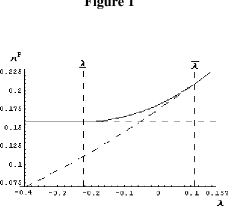
Unlike in Quirmbach’s (1992) model in which the dominant firm would choose full integration

unless it is arbitrarily restricted from doing so, the dominant firm does not necessarily want to

monopolize the downstream market when it is free to choose its degree of integration. Figure 1

portrays the predator’s profit as a function of λ when D(.) is linear, both R(.) and F(.) are cubic functions and R_DD >0 in the neighborhood of the equilibria. On the left of λ= −0.226, the upstream monopolist chooses not to be integrated, but it is partially integrated between λ and

0.111

λ= . For λ λ> , the fringe is ejected.7 Thus, an upstream monopolist with a cost

disadvantage in the downstream market may profitably integrate. Likewise, a predator that

enjoys a technological advantage over the fringe firms may prefer a partial integration scenario to

a monopoly scenario. The intuition behind these results is simple. Going back to the textbook

case involving downstream competitive firms with constant unit costs (i.e. F_xx =0 and F_qq =0), the predator is indifferent between integrating or not when λ=0, but would (not) integrate when

0

λ> (λ<0). In our model, the downstream market is an increasing cost one from the

perspective of the firms in the competitive fringe as well as the predator firm (i.e., F_xx >0 and

0

qq

F > ). As such, it is profitable for the predator to enter the market even when it has a cost

disadvantage and not to force the exit of the fringe when it has a cost advantage.

5

Implicitly defining λmax such that CP( )q =0, the domain for partial integration is λ∈

(

)

6

A different motivation for entry can be found in Blair, Cooper and Kaserman (1985).

7

As mentioned before, an increase in λ.can cause a non integrated upstream monopolist to

partial integrated the downstream market Hence, we may use static comparative to compare an

equilibrium without integration (λ λ= ) to one characterized by partial integration (λ λ> ).

Before dwelling on the welfare implications, we analyze the impact of partial integration upon

output and input prices.

Proposition 1: A) dp dλ<0. B) dr 0

dλ

>

< . A necessary, but not sufficient, condition for a cost

predation effect, dr 0

dλ > , is RDD >0. C) . 0

dp dr

dλ −dλ > if and only if RDD <2 /Dp <0.

Proof: Available upon request from the authors

Integration unambiguously induces a lower output price to the benefit of consumers, but it

has ambiguous effects on the input price and the fringe’s margin. If the upstream technology is

characterized by increasing returns such that R_DD <2 /D_p, then the integration makes the input

price fall enough to increase the fringe’s margin! To make sense of this result, note that the

condition on the upstream technology is derived under the assumption of increasing returns in the

downstream market. As a result, the predator firm may lower the input price to avoid moving up

too high on its output manufacturing marginal cost curve. Finally, the fringe’s output, like its

margin, may decrease or increase with λ.8

Proposition 2:A) ∂πP ∂ >λ 0, B) ∂πf ∂ >λ 0if and only if R_DD <2 /D_p <0, C) ∂CS ∂ >λ 0, and D) ∂W ∂ >λ 0.9

Proof: Available upon request from the authors.

Proposition 2 states that integration increases the predator’s profit, consumer surplus and

welfare. The fringe’s surplus can increase provided that there are sufficient economies of scale in

upstream production.

8

We obtain sign dS

(

( )

)

9_C

6. References

Blair, R. D., Cooper, T. E. and Kaserman, D. L. 1985. “A Note on Vertical Integration As

Entry.” International Journal of Industrial Organization, 3:219-229.

Church, J. and Ware, R. 2000. Industrial Organization: A Strategic Approach. Toronto:

Irwin-McGraw-Hill.

Quirmbach, H. C. 1992. “Sequential Vertical Integration.” Quarterly Journal of Economics, 107:

1101-11.

Riordan, M. H. 1998. “Anti-Competitive Vertical Integration by a Dominant Firm.” American

Economic Review, 88:1232-1248.

Salop, S.C. and Scheffman, D.T. 1987. “Cost-Raising Strategies.” The Journal of Industrial

Figure 1

Figure 1. The impact of λ on the predator’s profit when D p( ) 1= −p, _{R D( )}=_D3 _and 1

2