Comparison of Different Neural Network Architectures
for Classification of Feature Transformed Data for Face
Recognition
Amrita Biswas
Associate Professor,SMIT Majitar,Rangpo
East Sikkim
M.K.Ghose
Dean Academics,SMIT Majitar,Rangpo
East Sikkim
Moumee Pandit
Assistant Professor,SMIT Majitar,Rangpo
East Sikkim
ABSTRACT
In this paper neural network classifier is applied on transformed shape features for face recognition. Classification by neural networks to a large extent depends on the neural network architecture. We have investigated three different neural network architectures for classification namely-Feed Forward Neural Network, Cascade Feed Forward Neural Network and Radial Basis Function Neural Network and tested their performance for three sets of feature extracted data. For feature extraction we convert the 2-D gray level face images into their respective depth maps or physical shape which are subsequently transformed by three different methods to get three separate data sets,namely-Coiflet Packet , Radon Transform and Fourier Mellin Transform to compute energy for feature extraction. After feature extraction each of the training classes are optimally separated using linear discriminant analysis. The neural network classifiers have been tested on each of the three sets of feature extracted data and a comparative analysis has been done on the results obtained. The proposed algorithms have been tested on the ORL database, widely used for face recognition experiments.
General Terms
Pattern Recognition, Computer Vision, Artificial Intellegence,Image Processing
Keywords
Face Recognition,DWT,FMT,Radon Transform, Neural Networks, Radial Basis Functions
1.
INTRODUCTION
The use of face recognition systems largely in public and private places for access control and security, have attracted the attention of vision researchers for several years. Face recognition may seem an easy task for humans, and yet computerized face recognition system still cannot achieve a completely reliable performance. The difficulties arise due to large variation in facial appearance, head size, orientation and change in environment conditions. Such difficulties make face recognition one of the fundamental problems in pattern analysis. In recent years there has been a growing interest in machine recognition of faces due to potential commercial applications such as film processing, law enforcement, person identification, access control systems, etc. A recent survey of the face recognition systems can be found in references [1-2].
Several approaches for face recognition have been proposed so far. One of the most popular being the Eigen Face approach [3].The main idea of using PCA for face recognition is to
express the large 1-D vector of pixels constructed from 2-D facial image into the compact principal components of the feature space. Several researchers have applied neural network classification on eigen faces to compare the network performances[4-5].But the principal components of face image data gives no guarantee that this feature set is sufficient for better classification. Gabor wavelet transform is yet another popular approach in 2D face recognition problems [6-7].Several researchers applied neural network classification to Gabor filtered feature vectors. However, in practice, Gabor face responses have very long representation vectors and the dimension of Gabor feature vector is prohibitively large. In this paper we apply neural network classification techniques to transform based feature extracted data and features extracted are compact and the methods used are less time consuming.
The rest of the paper is organized as follows: In sec 2 the implemented face recognition algorithms are described in detail. In sec 3 a brief description of the three types of feature extraction methods used are given. In sec 4 the different types of neural network architectures used have been introduced .In sec 5 we provide the implementation and results obtained and finally conclude in sec 6.
2.
IMPLEMENTED FACE
RECOGNITION ALGORITHM
A standard face recognition system can be divided into three main parts:Data Preprocessing,Feature Extraction and Classification. Data Preprocessing involves steps like face detection, noise reduction, image resizing, scaling and so on.Feature Extraction involves extraction of data from the images that are relevant to face recognition and removal of any redundant data leading to reduction in size of the data set.Classification will involve determining the class of the input test data based on the features extracted from the training data set. In our work the first step preprocessing is not required because we have used the ORL database which consists of same sized noise free images. For Feature Extraction we have followed our previous research [8-9].
First the depth of all training images using shape from shading algorithm is computed.
To get the second data set the Radon transform followed by Fourier transform is applied to capture the directional features of the depth map images. The selected angle for Radon transform computation is θ, detected by the principal Eigen axis because of its uniqueness.
To get the third dataset the Fourier Mellin Transform of the depth images is computed [9].
For the obtained feature vectors the linear discriminant analysis is performed for better classification of data. For classification 3 different types of neural network architectures have been trained. Feed Forward Neural Network, Cascade Feed Forward Neural Network and Radial Basis Function Neural Network. In the next section we describe each of the above mentioned steps in details.
3.
FEATURE EXTRACTION
3.1
Shape from Shading
For our purpose, we have used the shape from shading algorithm described by P. S. Tsai and M. Shah [10] for its simplicity and speed. This approach employs discrete approximations for the surface gradients (p and q) using finite differences, and linearizes the reflectance in the depth map(Z(x,y)). The method is fast, since each operation is purely local. In addition, it gives good results for the spherical surfaces, unlike other linear methods. The illumination change may be due to the position change of the source keeping the strength of the source as it is or due to the change in the source strength keeping the position of the source fixed. In either case, the gradient values, p and q, of the surface do not change, i.e., they can be uniquely determined [11]. Hence, for the linear reflectance map, the illumination will have no effect on the depth map. In other words, depth map will be illumination invariant.
3.2
Discrete Wavelet Transform (DWT)
Wavelet transform has merits of multi-resolution, multi-scale decomposition, and so on. In frequency field, when the facial image is decomposed using two dimensional wavelet transform, we get four regions. These regions are: one low-frequency region LL (approximate component), and three high-frequency regions, namely LH(horizontal component), HL (vertical component),and HH(diagonal component), respectively. In wavelet packet decomposition [12], we divide each of these four regions in a similar way. To ensure almost nearly rotational invariance, the linear combination of the four subbands can be taken. This combination provides the sum of the different energy bands. For coiflets,this linear combination of four subband coiflet coefficients provides excellent constancy when the subject undergoes rotation. Also, note that coiflet has zero wavelet and zero scaling function moments in addition to one zero moment for orthogonality.As a result, a combination of zero wavelet and zero scaling function moments used with the samples of the signal may give superior results compared to wavelets with only zero wavelet moments [13].
3.3
RADON TRANSFORM
Due to inherent properties of Radon transform, it is a useful tool to capture the directional features of images.Therefore, Radon transform, computed with respect to this axis, tenders robust features. The Radon transform of a two dimensional function f(x,y) is defined as
dxdy
y
x
r
y
x
f
y
x
f
r
R
)
sin
cos
(
)
,
(
)]
,
(
)[
,
(
(1)
where
(.)
is the Dirac function,r
[
,
]
is the perpendicular distance of a line from the origin and]
,
0
[
[image:2.595.354.500.294.407.2]
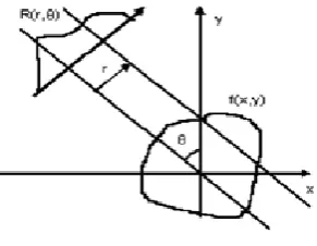
is the angle formed by the distance vector as shown in fig. 1.We have used Radon transform along the principal eigen axis given by the PCA method to compute the projections of all training images. Thus,the principal direction here is the direction of PCA eigen axis. The features so obtained are rotationally robust because the principal eigen axis, given by the PCA method, considers always the line that best fits the data cloud. Then their DFT magnitude may be taken to constitute the feature vectors. Thus, directional facial characteristics are incorporated in the feature values.Fig 1: Radon Transform
3.4
Fourier Mellin Transform (FMT)
The Fourier-Mellin Transform is often used for image recognition because the spectrum obtained after transformation is invariant in rotation, translation and scale. Translation invariance is already a property of Fourier Transform (FT) and when it is converted to log polar coordinates the scale and rotation differences are converted to vertical and horizontal offsets that can be measured. A second FFT, called the Mellin transform (MT) gives a transform space image that is invariant to translation, rotation and scale.
The AFMT can be expressed according to the Cartesian Coordinates of f as follows:
(2)
(3)
4.
CLASSIFICATION
Neural networks are composed of simple elements connected in parallel. These elements are inspired by biological nervous systems. As in nature, the connections between elements largely determine the network function. We can train a neural network to perform a particular function by adjusting the values of connections (weights) between the elements.
4.1
Feed Forward Neural Network (FFNN)
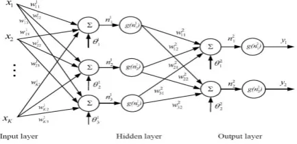
FFNN is a biologically inspired classification algorithm. It usually has a huge number of simple neuron-like processing units, which are arranged in layers. Every unit in a layer is linked with all the units in the previous layer. These connections are not all equal; each connection may have a different strength or weight. The weights on these connections encode the knowledge of a network. Data enters at the inputs and passes through the network, layer by layer, until it arrives at the outputs. During classification there is no feedback between layers. This is why they are called feed forward neural networks. A typical feed forward multilayer neural network is shown in fig.2 The inputs xn,k=1,……, N to
the neuron are multiplied by weights Wki and summed up
together with the constant bias term θi.The output yi, i=1,2, of
the network becomes
(4)
We can conclude that a multi layer feed forward neural network is a nonlinear parameterized map from input space
x∈RK to output space y∈Rm(here m = 3). The parameters are the weights wjik and the biases θjk.Activation functions g
usually assumed to be the same in each layer and known in advance. In Fig.2 the same activation function g is used in all layers. Given input-output data (xi,yi),i=1,….N is given as a
[image:3.595.63.280.613.718.2]data fitting problem.The parameters to be determined are the weights and biases(wjik,θjk).
Fig 2: Feedforward Multilayer Neural NetworkTraining Algorithm used: Scaled Conjugate Gradient Algorithm
The Scaled Conjugate Gradient Algorithm(SCG)algorithm is based upon a class of optimization techniques well known in numerical analysis as the Conjugate Gradient Methods[16]. SCG uses second order information from the neural network but requires only O(N) memory usage, where N is the number of weights in the network. The performance of SCG is benchmarked against the performance of the standard backpropagation algorithm (BP) [17], the conjugate gradient backpropagation (CGB) [18] and the one-step Broyden-Fletcher-Goldfarb-Shanno memoryless quasi-Newton algorithm (BFGS) [19].SCG yields a speed-up of at least an order of magnitude relative to BP. The speed-up depends on the convergence criterion, i.e., the bigger demand for reduction in error the bigger the speed-up. SCG is fully automated including no user dependent parameters and avoids a time consuming line-search, which CGB and BFGS uses in each iteration in order to determine an appropriate step size. The SCG algorithm is described as follows:
Let W is the weight vector,E(w) is the global error function depending on all the weights and biases , p1 ,..,pk, be a set of
non zero weight vectors in ℜN
(Weight Space) and the step size is αk
1. Choose initial weight vector w1
Set p1 = r1 = –E'(w1), k = 1.
2. Calculate second order information: sk = E''(wk)pk
δk = p T
ksk
3. Calculate step size: µk = pTkrk
αk = µk/δk
4. Update weightvector:
wk+1 = wk + αkpk
rk+1 = –E'(wk+1).
5. If k mod N = 0 then restart algorithm: pk+1 = rk+1
else create new conjugate direction:
βk =( |rk+1|2–rk+1rk)/µk
pk+1 = rk+1+ βkpk
6. If the steepest descent direction rk ≠ 0 then set k = k+1 and
go to 2
else terminate and return wk+1 as the desired minimum.
4.2
Cascade Feedforward Neural Network
(CFFNN)
architecture include a weight connection from the input to each layer and from each layer to the successive layers. For example, a three-layer network has connections from layer 1 to layer 2, layer 2 to layer 3 and layer 1 to layer 3. The three-layer network also has connections from the input to all three layers. The additional connections might improve the speed at which the network learns the desired relationship. Each neuron in the architecture includes weights, bias and a non-linear activation function. The weights of interconnections to the previous layer are called “input weights” and the weights of interconnections between the layers are called “link weights”. The commonly used hyperbolic tangent sigmoid activation function is used for all hidden layers while pure-linear function is used for output layer. A typical Cascaded architecture is shown in Fig. 3.The CFFNN network has been trained using the SCG Algorithm which is described in sec 4.1
Fig 3: Cascade Feedforward Multilayer Neural Network
4.3
Radial Basis Function Neural
Networks(RBFNN)
Radial basis neurons are used to classify data based on the center and variance of the Radial basis function. The increasing popularity of RBF neural networks is partly due to their simple topological structure, their locally tuned neurons and their ability to have a fast learning algorithm in comparison with the multi-layer feed forward neural networks [21].They are two-layer feed-forward networks. The hidden nodes implement a set of radial basis functions (e.g. Gaussian functions) and the output nodes implement linear summation functions as in multi layer feed forward networks. The network training is divided into two stages: first the weights from the input to hidden layer are determined, and then the weights from the hidden to output layer. The training/learning is very fast.
Where xi,i=1,..D,is the input vector,Φ(|| xP-x||) are a set of N
basis functions, one for each data point, where φ(.) is some non-linear function. The output of the mapping is then taken to be a linear combination of the basis functions, i.e.
[image:4.595.67.267.256.381.2](5)
Fig 4: Radial Basis Function Neural Network
5.
IMPLEMENTATION AND RESULTS
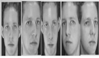
In order to test the proposed algorithms, the ORL(ATandT) database was used which contains 10 different images (92 x 112),each of 40 different subjects. All images were taken against a dark homogenous background with the subjects in upright, frontal position with some side movement. Sample images of the dataset are shown in Fig.5
Fig 5: Radial Basis Function Neural Network
Computing the Depth Map is common in all three feature extraction procedures. A sample image from the ORL Database with its depth map computed has been shown in fig.6
Fig 6: Depth Map from a sample image of the ORL Database
For the first feature extraction method using DWT size of each I/P training image is 112x92 and size of the feature vector obtained is 1x110.The obtained feature vectors are provided as I/P to the neural network classifier.
[image:4.595.342.514.326.426.2] [image:4.595.319.520.505.624.2]algorithm which is described in sec 4.1. We have trained the network for different numbers of training images for each class and have noted down the results in table 1.
Fig 7: 1st Level DWT Components Approximation, Horizontal Detail, Vertical Detail & Diagonal
Detail(Clockwise from top)
Next we have classified using the Cascade Feed Forward Neural Network.CFFNNs are similar to FFNNs, but include a connection from the input and every previous layer to following layers. As with feed-forward networks, a two-or more layer cascade-network can learn any finite input-output relationship arbitrarily well given enough hidden neurons.As before we have performed several experiments and selected a particular network configuration. The network has one i/p layer with no. of neurons= size of the i/p feature vector (which is 110 for the first dataset), 15 hidden layers with 2 neurons each and one o/p layer with no. of neurons=no.of classes being classified.Hyperbolic tangent sigmoid transfer function is used in the hidden layers and a linear transfer function is used in the output layer. The network was trained using the SCG algorithm.The results obtained for different training images is tabulated in table 1
Lastly we have classified using Radial Basis Function Neural Networks which can be trained considerably faster. Training has been done using the Orthogonal Least Squares Learning Algorithm(OLSL)[22].No. of i/p neuron is same as the size of the i/p feature vectors and the no.of o/p layers is equal to the no.of classes.Results are shown in table.1
Next the classification was performed on the data set obtained using Radon Transform followed by Fourier Transform.The size of each i/p training image is 112x92 and size of the feature vector obtained is 149x1.
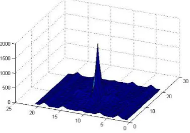
Fig. 8. Illustration of the Cartesian approximation of the AFMT of the image in Fig.7
For the Feed Forward Network we have selected one i/p layer with no. of nodes=110,5 hidden layers with no. of nodes =25 and one o/p layer with no.of nodes =No.of classes.Hyperbolic tangent sigmoid transfer function is used in the hidden layers and a linear transfer function is used in the output layer.Results shown in Table 2
For the Cascade Feed Forward Neural Network the i/p layer has 149 neurons, 15 hidden layers with 2 neurons each and one o/p layer with no.of classes being classified.Hyperbolic tangent sigmoid transfer function is used in the hidden layers and a linear transfer function is used in the output layer.Results in Table 2.
For the Radial basis networks no. of i/p neuron is same as the size of the i/p feature vectors and the no.of o/p layers is equal to the no.of o/p classes.Results are shown in table.2
Lastly the classification was performed on the data set obtained using Fourier Mellin Transform. For the Feed Forward Network we have selected one i/p layer with no. of nodes=size of feature vector which is 441,6 hidden layers with no. of nodes =40 and one o/p layer with no.of nodes =no.of classes.Hyperbolic tangent sigmoid transfer function is used in the hidden layers and a linear transfer function is used in the output layer.Results in Table 3.
For the Cascade Feed Forward Neural Network the i/p layer has 441 neurons, 15 hidden layers with 2 neurons each and one o/p layer with 10 neurons.Hyperbolic tangent sigmoid transfer function is used in the hidden layers and a linear transfer function is used in the output layer.Results in Table 3
[image:5.595.53.220.113.256.2]Table 1. Recognition % Obtained using DWT S l N o. No. of trai nin g ima ges /cla ss Reconi tion% using FFNN Trai ning Tim e Reconi tion% using CFFN N Trai ning Tim e Reconi tion% using RBFN N Trai ning Tim e
1 7 95 0:17 89 4:34 86 0:07
2 6 90 0:19 86 4:27 82 0:07
3 5 89 0:26 78 4:58 81 0:07
4 4 85 0:17 68 5:49 81 0:06
5 3 70 0:16 66 5:23 69 0:06
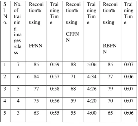
Table 2. Recognition % Obtained using Radon Transform
S l N o. No. of trai nin g ima ges /cla ss Reconi tion% using FFNN Trai ning Tim e Reconi tion% using CFFN N Trai ning Tim e Reconi tion% using RBFN N Trai ning Tim e
1 7 85 0:59 88 5:06 85 0:07
2 6 84 0:57 71 4:34 77 0:06
3 5 77 0:58 68 4:26 79 0:07
4 4 75 0:56 59 4:20 70 0:07
5 3 63 0:55 55 4:00 65 0:06
6.
CONCLUSION
From the above results we see that the best performance is provided by the DWT data set classified by the Feed Forward Neural Network. Performance is optimum in terms of the recognition percentage as well as the training time. From the results table we can infer that for all the three different sets of feature extracted data the Feed Forward Neural networks perform persistently well in terms of recognition percentage as well as training time. While CFFNN networks take longer time to train but do not provide as well recognition results. FFNN performs curve fitting operation in multidimensional space. Provided the network structure is sufficiently large (i.e sufficient no.of hidden neurons) any contiguous function can be approximated to within an arbitrary accuracy by carefully choosing parameters in the network. An RBFNN network can be considered as a special case of two layer neural network. From the results obtained it can be inferred that though the training time of RBFs are significantly less than FFNNs but the FFNNs performs better in terms of recognition percentage
[image:6.595.309.548.135.365.2]than the RBFs.Also for RBFNNs the recognition percentage falls drastically with the reduction in number of training images.
Table 3. Recognition % Obtained using Fourier MellinTransform S l N o. No. of trai nin g ima ges /cla ss Reconi tion% using FFNN Trai ning Tim e Reconi tion% using CFFN N Trai ning Tim e Reconi tion% using RBFN N Trai ning Tim e
1 7 90 0:23 86 5:20 87 0:08
2 6 88 0:14 79 6:21 71 0:08
3 5 83 0:29 69 4:41 74 0:07
4 4 70 0:17 63 5:36 70 0:06
5 3 65 0:16 60 4:07 63 0:07
7.
REFERENCES
[1] Rabia Jafri and Hamid R Arabina, “A survey of Face Recognition Techniques”,Journal of Information Processing Systems,Vol.5,No.2,June 2009
[2] W. Zhao, R. Chellappa, P. J. Phillips, “A. Rosenfeld,FaceRecognition:A Literature Survey”,ACM Computing Surveys, Vol. 35, No. 4,pp.399-458.,2003
[3] Hyeonjoon Moon, P Jonathon Phillips,“Computational and Performance Aspects of PCA Based Face Recognition Algorithms”, Perception 30(3),pp.303 - 321,2001
[4] Meftah Ur Rahman, “A comparative study on Face Recognition Systems and Neural networks”Computer Vision and Pattern Recognition,arXiv:1210.1916v1,2012
[5] P.Latha,Dr.L.Ganesan,Dr.S.Annadurai, “Face Recognition using Neural networks”, Signal Processing: An International Journal (SPIJ) Volume (3) : Issue (5),pp 153-160
[6] Anissa Bouzalmat, NaouarBelghini, ArsalaneZarghili, Jamal Kharroubi&AichaMajda,”Face Recognition using Neural network based Fourier Gabor Filters & Random Projection”,International Journal of Computer Science and Security,(IJCSS),Vol.5,Issue.3,2011
[7] V. BalamuruganMukundan Srinivasan Vijayanarayanan. A,”A New Face Recognition Technique using Gabor Wavelet Transform and Back Propagation Network”,International Journal of Computer Applications,Vol.49,No.3,2012
[8] Sambhunath Biswas and Amrita Biswas,“Face Recognition Algorithms Based on Transformed Shape Features“, IJCSI International Journal of Computer Science Issues, Vol. 9, Issue 3, No 3, pp-445-451,May 2012
[image:6.595.48.287.335.552.2]of Computer Engineering and Technology(IJCET),vol.4,issue 1,pp8-15,2013
[10] Ping-Sing Tsai and Mubarak Shah “Shape From Shading Using Linear Approximation”, Image and Vision Computing,vol:12, pp.487-498,1994
[11] B.K.P Horn,” Robot Vision”, Cambridge,Massachusetts, USA ,MIT Press,1986.
[12] R. C. Gonzalez and R. E. woods,” Digital Image Processing”, Dorling Kindersley, India, Pearson Prentice Hall, 2006.
[13]C.SydneyBurrus and A. Gopinath and HaitaoGuo,“Introduction to Wavelets and Wavelet Transforms”,Prentice Hall, N.J 07458, USA, 1998.
[14] St´ephaneDerrode,Robust and Efficient Fourier–Mellin Transform Approximations for Gray-Level Image Reconstruction and Complete Invariant escription Computer Vision and Image Understanding 83, 57–78 (2001)
[15] KouroshJafari-Khouzani and Hamid Soltanian-Zadeh,RadonTransformOrientation Estimation For Rotation Invariant Texture Analysis, IEEE Trans. on Pattern Analysis and Machine Intelligence, vol. 27, no. 6, June2005.
[16]Martin Fodslette Moller “A Sacled Conjugate Gradient Algorithm for Fast Supervised Learning”, Neural Networks, Vol. 6, pp. 525-533, 1993
[17]Rumelhart, D.E., G.E. Hinton, R.J. Williams,”Learning Internal Representations by Error Propagation, in:
Parallel Distributed Processing”, Exploration inthe Microstructure of Cognition, Eds. D.E. Rumelhart, J.L. McClelland, MIT Press,Cambridge, MA., pp 318–362, 1986.
[18] Johansson, E.M., F.U. Dowla, D.M. Goodman, “BackpropagationLearningfor Multi-Layer Feed-Forward Neural Networks Using the Conjugate Gradient Method”,Lawrence Livermore National Laboratory, Preprint UCRL-JC-104850, 1990.
[19] Battiti, R., F. Masulli, “BFGS Optimization for Faster and Automated Supervised Learning”, INCC 90 Paris, International Neural Network Conference, pp 757– 760,1990.
[20] Dheeraj S Badde,Anil K Gupta,Vinayak K Patki,”Cascade and Feedforward Neural Network Backpropagation Models for Prediction of Compressive Strength of Ready Mix Concrete”, IOSR Journal of Mechanical and Civil Engineering (IOSR-JMCE) ISSN: 2278-1684, PP: 01-06
[21] Meng Joo Er, Shiqian Wu, Juwei Lu, Hock Lye Toh,”Face Recognition with Radial Basis Function Neural networks”, IEEE Transactions On Neural Networks, Vol. 13, No. 3, May 2002