Exploring New Angles to Analyze Student Load Data
Amir H. Rouhi
RMIT University Melbourne, Australia
Copyright©2018 by authors, all rights reserved. Authors agree that this article remains permanently open access under the terms of the Creative Commons Attribution License 4.0 International License
Abstract
Over the past 25 years, performance measurement has gained salience in higher education, and with the explosion of structured data and the impact of business analytics and intelligence systems, there are new angles by which big volumes of data can be analyzed. Using traditional analytical approaches, pairs of reciprocal cohorts are considered as two separate discrete entities; therefore, basis of analysis are individual pairs of values, using statistical measures such as average, mean or median, of the total population. Missing in traditional approaches is a holistic performance measure in which the shape of the comparable cohorts is being compared to the overall cohort population (vector-based analysis). The purpose of this research is to examine shape analysis, using a Cosine similarity measure to distil new perspectives on performance measures in higher education. Cosine similarity measures the angle between the two vectors, regardless of the impact of their magnitude. Therefore, the more similar behavior of the two comparing entities can be interpreted as more similar orientation or smaller angle between the two vectors. The efficacy of the proposed method is experimented on the three Colleges of RMIT University from 2011 to 2016, and analyzes the shape of different cohorts. The current research also compared the performance of Cosine similarity with two other distance measures: Euclidean and Manhattan distance. The experimental results, using vector-based techniques, provide new insights to analyzing patterns of student load distribution and provide additional angles by orientation instead of magnitude / volume comparison.Keywords
Student Load Pattern Distribution, Vector-based Analysis, Shape Analysis, Cosine Similarity1. Introduction
Australia’s higher education system has undertaken many successive market-driven reforms since the late 1980s. These reforms together with the increased democratization of education both in terms of student participation and increased provision through institutional
diversification has provided an impetus for greater utilization of the statistical information that institutions collect, and to better inform institutional decision making. Australia has had a robust and comprehensive data collection for many decades and that has enabled institutional researchers and planners undertake analysis of the vast amounts of data that is collected (Calderon 2015; Borden et al. 2013).
With respect to the growth of stored structured data in educational organizations, specifically in higher education, the use of modern analytical tools that provide a holistic analysis of student load or headcount data is in increased demand due to competitive forces influencing higher education. For this analysis we make use of the term student load, and it is a measure that counts students in terms of full-time equivalence units (EFTSL). In the view of the Australian Department of Education an “EFTSL is an equivalent full-time student load for a year. It is a measure, in respect of a course of study, of the study load for a year of a student undertaking that course of study on a full-time basis’ (Department of Education and Training nd).
Conventional student load analysis is basically comparing pairs of reciprocal cohorts which are summarized in the form of “Average” or “Sum” of series of data. The essence of such approaches is based on scalar interpretation which focuses on magnitude of results (Ma. Florecilla et al. 2017). However, scalar-interpretation analysis suffers from lack of vector information which represents the holistic similarity in distribution (shape) of compared data. As an example, trend analysis of educational load in consecutive years is useful to investigate the overall performance but does not represent the organizational load pattern. Or how to investigate the impact of policy changes in the performance of Colleges and schools, regardless of comparing their performance magnitude only.
Vector-based approach is utilized in image analysis to investigate the content-based similarity (distance) among the images. Images are 2-dimensional data in form of integer matrices. We applied a similar approach on 1- and 2-dimensional data to investigate the similarity of performance in consecutive years or semesters. Shape analysis is a term which is applied to this approach in the current research.
Two models are proposed in this research: Cosine similarity and Minkowsky distances (Euclidean and Manhattan). These two distance metrics are utilized in image analysis to investigate the similarity between content of images.
The data utilized in this research is provided by RMIT University from 2010 to 2016. The total performance and shape analysis of a sample College of RMIT University is investigated in this research.
In the next section, we introduce background and related works of the proposed method in detail. Methodology of shape analysis of load data is introduced in the third section. The fourth section is dedicated to the scalar versus vector analysis. The fifth Section is dedicated to analyzing the results and discussions for the two shape analysis models and finally the sixth section represents the conclusion of the current research.
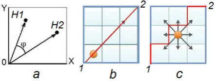
Figure 1. Cosine similarity between two vectors: H1 and H2 by measuring the cosine of the Φ angle. The Euclidean and Manhattan distances between two points are shown in (b) & (c) respectively.
This analysis provides an alternative lens by which institutional planners can further explain to decision makers’ changes in the student distribution as well as considering its effect on various cohorts. The other critical outcome of this research is that it challenges traditional approaches for examining student load distribution over time, and it suggests new possibilities that can be considered, e.g. where opportunities for growth in certain market segments have been inadvertently missed.
2. Background and Related Works
To measure the similarity between two vectors, measuring the cosine of the angles between the two vectors is a method known as cosine similarity (Huang 2008, Ye 2011). The range of result is between -1 and 1. If the angle is zero, it shows the ultimate similarity between the two compared vectors, regardless of their magnitude, which the cosine similarity would be 1. Conversely when the twovectors are totally in opposite directions, the cosine angle would be -1. Two vertical vectors represent 0 similarities in this approach. Figure 1-a illustrates the cosine similarity between two vectors and Formula 1 shows how to calculate this similarity measure.
𝐶𝐶𝐶𝐶𝐶𝐶(𝐻𝐻1,𝐻𝐻2) =‖𝐻𝐻1‖.‖𝐻𝐻2‖𝐻𝐻1.𝐻𝐻2 𝑆𝑆(𝐻𝐻1, 𝐻𝐻2) = ∑𝑛𝑛𝑖𝑖=1(𝐻𝐻1𝑖𝑖𝐻𝐻2𝑖𝑖)
�∑𝑛𝑛𝑖𝑖=1𝐻𝐻12𝑖𝑖�∑𝑛𝑛𝑖𝑖=1𝐻𝐻2𝑖𝑖2 (1) Formula 1 shows the cosine of the angle between two vectors H1 and H2 is equal to the dot product of the two vectors divided by the magnitude of them. The formula is expanded in S(H1, H2) where S represents the similarity of vectors H1 and H2. The components of the vectors are shown as H1i and H2i.
[image:2.595.63.286.386.470.2]There are other distance measures to investigate the similarity among two vectors (Rouhi 2015). Minkowski distance measures the distance between the two points or vectors. Two of the most popular Minkowski distances are Euclidean and Manhattan distance metrics (Huang 2008). To simplify the concept we can focus on the distance between two points in a 2-dimensional plane. Euclidean or L2 Norm, measures the straight line between the two points. Calculation of this distance is shown in Formula 2.
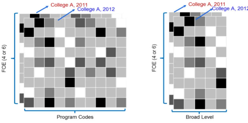
Figure 2. Content of an image in two modes; top in a colored image and bottom in a grey-level image
𝐸𝐸𝐸𝐸(𝐻𝐻1, 𝐻𝐻2) = �∑ (𝐻𝐻1𝑛𝑛𝑖𝑖=1 𝑖𝑖− 𝐻𝐻2𝑖𝑖)2 (2) If H1 and H2 represent two vectors, the Ed (Euclidean distance) between the two vectors would be equal with the sum of squares of the differences of the corresponding components. The resulting value shows the straight distance between the two vectors or points. Figure 1-b shows Euclidean distance between two points: 1 and 2.
For the same situation, the Manhattan distance represents the distance between the two vectors or points but strictly on horizontal and vertical paths, unlike Euclidean which utilizes the diagonal path. Figure 1-c and Formula 3 represent this distance.
[image:2.595.309.534.389.509.2]seen in Figure 1-c, the Manhattan distance is the simple sum of horizontal and vertical distances between two points in a 2-dimensional plane.
One of the applications of cosine similarity and Minkowski distances are in content-based image processing (Russ 2016). Colored images are composed of three tables or matrices that contain integer values, representing the intensity of light for three basic color components: Red, Green and Blue. The same concept is used for grey-level images. The only difference is that grey level images utilize only a single matrix to store the intensity of light; 0 for black and 255 for white components which are known as pixels, unlike the colored images which are composed of three matrices. The integer values between 0 and 255 represent the different shades of grey (Hau 2015, Russ 2016). Figure 2 demonstrates the concept of colored (top) and grey-level (bottom) image.
As depicted in Figure 2, an image is nothing more than matrices of integer values. Hence, the techniques that compare two images by calculating the similarity or distances between the two images can be used for any data which is represented as 2-dimensional vectors (tables). The authors of the current research utilized the idea from the content-based image similarity detection and implemented the models on educational student load data. The results show the cosine similarity can be utilized as a holistic performance measure or shape analysis tool in analysis of educational data. The details will be presented and discussed in the fifth section.
3. Sample Applications
As described in the previous section, a grey-level image is just an integer matrix. If similarity between the images can be implemented by help of mathematical distance
measures, utilizing the same methods can therefore be implemented on any numeric matrices i.e. Actual student load, Target student load and Enrolment headcount of different cohorts in educational data warehouses.
3.1. Student Load Analysis of a College/University
To provide a platform for evaluating the proposed models for shape analysis, the performance of a college at RMIT University was selected as the pilot platform. A common approach is measuring the performance of the selected college by comparing scalar values representing student load (or headcount). However this approach is incapable of evaluating the similarity on load pattern distribution of the specified college which represents the college shape.
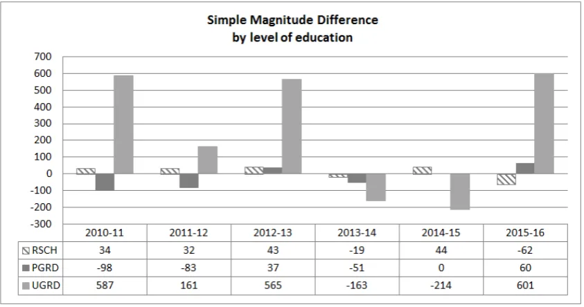
To achieve this, the college student load data should be composed in the form of a matrix (table) for each year. The X-axis of the matrix can represent the Broad-levels of education (BLEVEL) or program codes and the Y-axis can represent the broad or narrow Fields of Education (FoEs). In such a composition, each element of the matrix represents the total student load of each Blevel or program by FoEs (narrow or broad).
Providing the same matrix for each year of the college performance finally generate several matrices with similar number of rows and columns. It should be noted that if a FoE or Blevel or program does not exist in some years, it should appear in those matrices with zero values to make all matrices equal in size, similar number of rows and columns. Figure 3 illustrates student load distribution for a sample college in the two compositions; FoEs (narrow or broad) by programs (left) and FoEs (narrow or broad) by Blevels (right). The experiments conducted in the current research are based on narrow FoEs by Blevels.
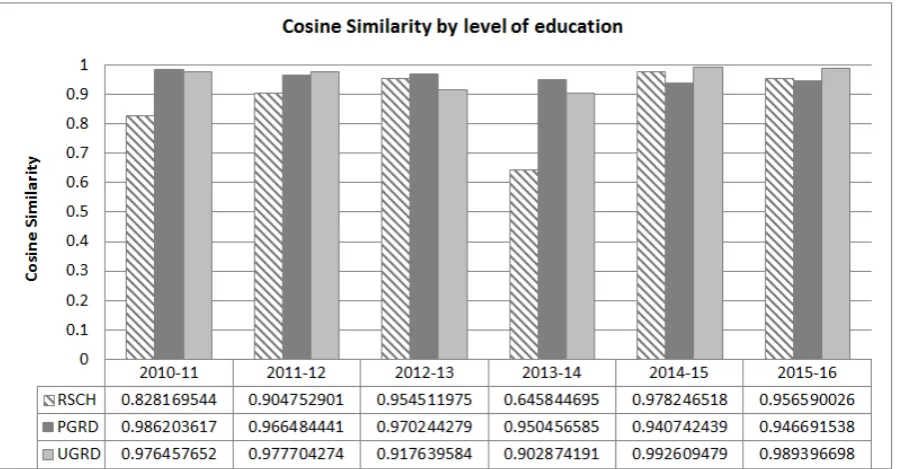
[image:3.595.88.506.518.725.2]Figure 4. Conventional performance analysis of a sample college based on sum of load difference
Table 1. Total sum of student load for the sample college breakdown by Blevel and year
Year RSCH PGRD UGRD Total(Year)
2010 181 1542 4112 5835
2011 215 1444 4699 6358
2012 247 1361 4860 6468
2013 290 1398 5425 7113
2014 271 1347 5262 6880
2015 315 1347 5048 6710
2016 253 1407 5649 7309
[image:4.595.57.537.458.712.2]Total (Blevel) 1772 9846 35055
Table 2. Detailed load table of the sample college breakdown by narrow FoE, Blevel and year narrow
FoE Blevel RSCH PGRD UGRD RSCH Year 2010 PGRD 2011 UGRD RSCH PGRD UGRD RSCH … PGRD 2016 UGRD
010101 2 0 35 3 0 54 ... ... ... 0 0 34
010103 0 20 14 1 30 23 ... ... ... 0 104 23
010301 5 0 9 14 0 6 ... ... ... 21 19 8
… … … …
061999 0 9 0 0 13 0 ... ... ... 0 7 0
090799 0 7 0 0 17 0 … … … 3 7 213
Total 181 1542 4112 215 1444 4699 … … … 253 1407 5649
3.1.1. Scalar- Versus Vector-based Student Load Analysis The student load (EFTSL) of a sample college at RMIT University has been selected to evaluate the proposed methods for shape analysis in different years. The three Blevels for each year are as follows:
Higher degree by research programs (RSCH)
Postgraduate by Coursework programs (PGRD) and
Undergraduate programs (UGRD).
The original data is in the format of load by year and Blevel, presented in Table 1. Student load of each year is presented in format of a list (1-dimensional) of values in rows and columns. This format is normally used in conventional analysis models (Tinto 2006, Kuh 2008).
The simple data structure in Table 1 is broken down by narrow FoEs and each year is represented as a matrix (2-dimensional) showing the load of FoEs by Blevels as shown in Table 2 partially.
To investigate the performance of the specified college in each Blevel, the conventional model is comparing the sum of Blevels in each year. The graph shown in Figure 4 illustrates the difference of the overall load, presented in Table 1, broken down by Blevels, by years. This approach can help us to analyze the trend and investigate about the performance growth rate.
[image:5.595.74.523.451.685.2]However conventional models are incapable of analyzing the student load based on the load pattern distribution. Such load distribution is demonstrated in Table 2 in the form of a list (colored columns) or sub-tables
(tripled-line matrices) as well as in Figure 5. This characteristic is called Shape Analysis in this research and investigates the similarity of load pattern distribution in the columns or sub-tables of Table 2. Figure 5 depicts the student load distribution used for shape analysis in 1-dimensional (4-a) and 2-dimensional (4-b) models. To compute shape analysis for Blevels, the cosine similarity, introduced in Formula 1, is used. In this approach each two comparable Blevels, i.e. 2010-RSCH and 2011-RSCH, are considered as two vectors: H1 and H2 which are highlighted in the same color in Table 2. Applying the cosine similarity provides the angle between the two vectors, regardless of their overall magnitude.
The similarity in student load pattern is represented by similar increase or decrease of load in the corresponding pairs of FoEs, which finally represents similarity in the behavior of the specified college. The core competency of shape analysis is in vector interpretation of data which is independent of the overall magnitude of load in each category (scalar interpretation).
3.1.2. Results and Discussion
In this section a detailed comparison between the conventional and the proposed models is provided and discussed in two sub-sections. The first model provides a 1-dimensional load analysis of the sample college on each Blevel. However the second model provides 2-dimensional load analyses of the college in a holistic approach including all the Blevels.
3.1.2.1. Cosine-similarity Model for 1-dimensional Student Load Analysis
The conventional student load analysis on Blevels is based on the difference of overall magnitude of Blevels on pairs of years. The results of this method are demonstrated in Figure 4 which is derived from the sum of loads provided in Table 1. As an example, for UGRD load analysis based on the conventional model, Figure 4 reveals that the maximum load reduction can be seen in the 2014-15 years with negative growth of -214 EFTSL.
Conversely for the same UGRD programs, the maximum increase of load can be seen in 2015-16 with positive growth of +614 EFTSL. Based on the conventional model, the most significant fluctuation of UGRD programs can be seen in these two pairs of years.
[image:6.595.91.509.282.493.2] [image:6.595.86.508.531.730.2]The proposed model based on cosine similarity shown in Figure 6 reveals another aspect which does not conform to conventional load analysis shown in Figure 4. The graph in Fig (5) shows the UGRD programs in the same paired years (2014-15 and 2015-16), have a cosine similarity near to 1, which reveals the shape of the college has been almost identical in those pairs of years. The cosine similarity value for UGRD programs in 2014-15 and 2015-16, is 0.99 and 0.98 respectively which shows the angle between the two vectors is almost zero, similarly for 2015-UGRD and 2016-UGRD. From an analytical point of view, the higher values in cosine similarity represent the lower changes in distribution of load among compared pairs of cohorts. It shows that the college has similar pattern in increasing or decreasing of load among UGRD FoEs. In other words, the college behaves in similar shape for UGRD programs.
Figure 7. Comparing pairwise student load of a sample college by Euclidean (solid-bars) versus conventional sum of load (crossed-bars) from 2010 to 2016.
Another example is the RSCH programs in 2013-14. The overall magnitude in RSCH programs, between RSCH-2013 and RSCH-2014 is -19 which is the lowest. Conversely the college shows the maximum change in its shape due to minimum value of cosine similarity: 0.64, compared to the previous and following years. This can be the result of offering new FoEs or significant load change in some of the research programs in the FoEs of these two years.
As can be seen in Figure 5-a, this model analyzes the distribution of student load by Blevels individually and consequently the magnitude of load among Blevels does not skew the analysis results.
The significant aspect of the proposed model is its independency of overall sum of load. Such tolerance against the load magnitude is the core competency of the proposed shape analysis based on cosine similarity. This model is general and can be applied on any cohorts such as analyzing the shape of load distribution of:
Low-SES versus other domestic students,
International versus domestic,
ATSI versus domestic and
Gender student load distributions.
3.1.2.2. Minkowski-distances Models for 2-dimensional Student Load Analysis
The experiments of this section are conducted on the same college used for cosine similarity. However instead of comparing the individual Blevels comparisons, we compared the holistic college performance on all the three Blevels for pairs of consecutive years. The results are shown in Figure 7 and 8. In both figures the overall load difference is compared with the Minkowski distances.
Two Minkowski distance measures will be introduced in this section: Euclidean and Manhattan. Both distances have similar behavior and naturally show the same distribution of load but with different scales. The results of these distance measures are positive values and represent the distance among student load pattern distribution of the two compared entities. These measures are incapable of detecting which compared cohorts are higher or lower, but they can show how their shapes are following a similar load pattern distribution on FoEs.
The conventional model shows the maximum student load difference of the college can be seen in 2012-13 (645), 2015-16 (599) and 2010-11 (523). However, the proposed 2-dimensional models focus on distribution of load within the matrices of each year as shown in Figure 5-b. These models show the largest distance between the shape (load pattern distribution on all narrow FoEs) of the college can be seen in 2013-14 while its magnitude in the conventional model is insignificant (-233). The reasons for such shape difference can be due to introducing new programs or fluctuation in FoEs load which can justify the larger Minkowski distances of 2013-14.
This contrast between the conventional approach and the Minkowski distances helps decision makers better interpret
and analyze holistic college performance. Similarly, these models can be applied on any cohorts as mentioned in the previous section.
3.2. Analyzing the Process of Student Load Targeting Student load targeting for future years of a program is a routine procedure for those engaged in institutional planning in higher education. The procedure generally utilizes regression techniques over past several years of student load data and then generates targets for student load in each program for the following years. In this research two approaches were experimented as follows:
Pairwise analysis of actual versus actual loads of consecutive years plus the target load in 2018, and
Pairwise analysis of actual versus target load of the same years.
Both approaches utilized cosine similarity method on student load (actual and target) to evaluate the two different aspects of load targeting process.
3.2.1. Pairwise Analysis of Actual versus Actual Load of Consecutive Years
To analyze the trend of student load in this approach, a dataset including 4 years of load data were provided. The dataset includes three years of actual student loads as well as target load of future year (2018). The loads are grouped by three cohorts (Blevels: UGRD, PGRD and RSCH) and are compared for two colleges (A, B). Figures 9, 10 and 11 illustrate magnitude difference on actual load on pairs of years for the two sample college.
To analyze the student load a pairwise comparison of subsequent years was implemented. This is done by comparing the pattern distribution of student loads, by each program in each cohort, to the same programs in the paired year, using cosine similarity. The similarity measures are shown in % with the orange line in the graphs. The higher similarity measure represents the more similar distribution of loads among pairs of identical programs on the two compared years.
Since the charts represent the trend of the actual loads and target of the future year, they can potentially provide more insight for decision makers. The analytical finding for each cohort is provided as follows:
3.2.1.1. Pairwise Analysis of Actual Student Loads for Research Programs (Figure 9)
Figure 9. Cosine similarity on magnitude of student load in research cohort of college_A and _B. The bars represent the actual load differences on pairs of years: 2015-16, 2016-17 and 2017-18 (2018 targets).
Figure 10. Cosine similarity on magnitude of student load in postgrad cohort of college A and B. The bars represent the actual load differences on pairs of years: 2015-16, 2016-17 and 2017-18 (2018 targets).
3.2.1.2. Pairwise Analysis of Actual Student Loads for Postgraduate Programs (Figure 10)
College_A shows a steady increase in load of postgraduate programs from 2015 onward. The increase of load in 2018 is not identical with 2017. 96% of the programs loads show similar increases in 2018 compared to 2017. College_B shows a steady increase in postgraduate programs from 2015 onward. The increase of load in 2018 is almost identical with 2017 (99%). However the load distribution did not evenly increase in 2015-16 and 2016-17. It can be interpreted as satisfaction of college_B with the student load distribution in postgraduate programs in 2017 and just increasing their load magnitude identically for 2018 targets.
3.2.1.3. Pairwise Analysis of Actual Student Loads for Undergraduate Programs (Figure 11)
[image:8.595.71.526.303.490.2]Figure 11. Cosine similarity on magnitude of student load in undergrad cohort of college_A and _B. The bars represent the actual load differences on pairs of years: 2015-16, 2016-17 and 2017-18 (2018 targets).
Figure 12. Cosine similarity on magnitude of actual and target student load of each year of research programs in two colleges: A and B. The solid bars represent actual and the grid bars represent target load on pairs of years: 2012 to 2017. The similarity of student loads by programs in actual and target is shown by line chart.
3.2.2. Pairwise Analysis of Actual versus Target Student Load of the Same Years
The proposed similarity measure can be used as a tool to analyze the process of program load targeting. A set of historical data including pairs of actual and target load are provided for this analysis. The results are shown in the following graphs. Unlike the previous graphs which show single values representing the magnitude of the student load differences, these figures show a pair of values for each year: actual and target load. The cosine similarity measured the distance between the actual and target load for each year separately and are depicted by line charts.
The dataset covers the actual and target load by programs from 2012 to 2017. The detailed student load data is summed into three major cohorts (Blevels: UGRD, PGRD and RSCH) and are compared for two colleges (A, B), similar to the previous analysis in 2-1. The results are shown in Figures: 12, 13 and 14. The analysis of the data for each cohort is as follows:
3.2.2.1. Analysis of Actual versus Target Student Load in Research Programs (Figure 12)
College_A shows a steady increase in target and actual load in research programs from 2012 to 2015. The distribution of student loads between actual and target program lists are not identical and show a similarity range from 93% to 96% which represents the improvement in load targeting of research program in college_A. The scenario changed in 2016 and 2017. In spite of a steady increase in target loads, the actual load decreased. However the load targeting process absolutely improved and shows 100% similarity between distribution of target and actual load. An interpretation for such behavior in college A is improving the load targeting process in a way that actual and target load steadily improved from 93% to 100% from 2012 to 2017, although with lower in actual student loads in the last two years.
[image:9.595.70.525.304.469.2]the 6 years. The significant phenomenon is the similarity in the distribution of student load between actual and target loads in 2014 which is almost 0%. Further investigation revealed that this phenomenon occurred due to massive research program code changes in 2014 in college_B. Consequently the new program codes in actual loads could not be matched with the student loads in the target list which was designed based on old program codes. The improvement in the targeting load process of research program can be seen in this college as well.
3.2.2.2. Analysis of Actual versus Target Student Load in Postgraduate Programs (Figure 13)
In college_A and _B a similar pattern can be seen in
[image:10.595.73.526.272.428.2]postgraduate programs, but in two different scale and time slices. College_A had an increase in actual loads from 2012 to 2014, although the target loads for these years had not precisely predicted. The worst targeting process was in 2014. However such significant dissimilarity forced the college_A team to optimize their student load targeting process and the results can be seen in the consequent years. The similarity between target load and actual load shows a steady increase from 2015 with 94% to almost 100% in 2017. However the actual load in 2017 show more than that targeted but definitely in a similar pattern of student load. The same scenario can be seen on postgraduate programs of college_B. The only difference is in the time that the load targeting issue occurred.
Figure 13. Cosine similarity on magnitude of actual and target student load of each year of postgraduate programs in two colleges: A and B. The solid bars represent actual and the grid bars represent target load on pairs of years: 2012 to 2017. The similarity of student loads by programs in actual and target is shown by line chart.
[image:10.595.72.526.479.646.2]3.2.2.3. Analysis of Actual versus Target Student Load in Undergraduate Programs (Figure 14)
College_A and _B show steady increases in target and actual student load in undergraduate programs from 2012 to 2017. The load targeting process for undergraduate programs shows almost 100% similarities with actual loads. The only significant drop in similarity of actual and target student loads can be seen in college_A in 2014. Possible reason for such a drop can be because of minor program code changes or because of a deficiency in load targeting process in 2014.
4. Conclusions
The objective of this research is to introduce new models to analyze quantitative data in education systems. The proposed approach utilizes vector- instead of the scalar-based interpretation used in the conventional analysis models (Tinto 2006, Kuh 2008, Ye 2011, Ma. Florecilla et al. 2017).
The utilized distance measures have been used in image processing to measure the content-based similarity among the images. Since an image is a matrix of integer values (intensity of pixels), the idea inspired us to utilize the same techniques for analyzing the educational load data which is configured in the form of a matrix.
Two models are introduced: Cosine similarity and Minkowski distances (Euclidean and Manhattan) for partial and holistic shape analysis. The efficacy of the methods was investigated on two applications:
Analysis of the student load data of a sample college in RMIT University from 2010 to 2016. The results show the capability of the proposed techniques in analyzing load pattern (shape) of the college by comparing the distribution of loads by Field of Educations (FoEs) and Broad-levels or Education (Blevels).
Analysis of target load data in two approaches. The actual and target student load data of two sample colleges in RMIT University was utilized for this section. The focus of the first approach was based on comparing the actual student loads on pairs of consecutive years including the target load of future year and comparing the similarities and magnitudes on pairs of years. The second approach compared the actual and target loads in each year and investigated the similarities between the load distributions on the two lists of each year.
The proposed shape analysis models can help decision makers to answer some questions such as; how similar is the load pattern of an educational cohort to the other cohorts or compared to itself during the previous years, or how similar is the shape of actual student load data with target student load in educational organizations. Another application which is not investigated in this paper would be
to investigate the similarity of a college or a University with other colleges or Universities.
Analyzing the distribution of student load and measuring it with the proposed models, can help educational organizations to investigate their performance from a new angle and provide more insights to decision makers to develop more effective strategies. For example, the utilization of this approach could lead to a shift in student recruitment away from historical patterns to one where new possibilities are considered. For decision-makers this new approach could provide a new validation angle by which student load distribution data can be put to
hypothesis-testing or forecasting.
Acknowledgment
We thank Kate Reale and Sean Lee for their sincere support; Chris Van Zeyl for providing timely guidance about the scope and completeness of the data, and Barbara Sainsbery for her editorial assistance.
REFERENCES
[1] Hau, C. C. (2015). Handbook of pattern recognition and computer vision, Chapter: Basic Methods in pattern Recognition, Sec: Statistical pattern recognition, World Scientific.
[2] Borden, V., Calderon, A., Fourie, N., Lepori, B., & Bonaccorsi, A. (2013). Challenges in developing data collection systems in a rapidly evolving higher education environment. In A. Calderon & K. L. Webber (Eds.), Global issues in institutional research (pp. 39-57). New Directions for Institutional Research, No. 157. San Francisco: Jossey- Bass.
[3] Calderon, A. (2015). In light of globalization, massification and marketization: Some considerations in the use of data in higher education. In Webber, K. L. and A. J. Calderon (Eds.) Institutional research and planning in higher education. Global contexts and themes. (pp. 186-196), Abingdon, UK and New York, NY: Routledge.
[4] Departmen of Education and Training. n.d. Equivalent Full-Time Student Load. Retrieved from: http://heimshelp.education.gov.au/sites/heimshelp/2014_da ta_requirements/2014dataelements/pages/339
[5] Huang, A. (2008). Similarity measures for text document clustering. Proceedings of the sixth New Zealand computer science research student conference (NZCSRSC2008), Christchurch, New Zealand.
[6] Kuh, G. D., et al. (2008). Unmasking the effects of student engagement on first-year College grades and persistence. The Journal of Higher Education 79(5): 540-563.
Research in South East Asia 15(1).
[8] Rouhi, A. H. (2015). Evaluating spatio-temporal parameters in video similarity detection by global descriptors. Digital Image Computing: Techniques and Applications (DICTA)(International Conference on. IEEE): 1-8.
[9] Russ, J. C. (2016). The image processing handbook, Chapter: Processing Binary Images, Sec: Euclidean
Distance Map, CRC press.
[10] Tinto, V. (2006). Research and practice of student retention: What next? Journal of College Student Retention: Research Theory & Practice (8.1): 1-19.