Multi baseline SAR Interferometry using Elaboration of Amplitude and Phase Data

Multi-baseline SAR Interferometry using Elaboration of

Amplitude and Phase Data

Carmine Abbate

1,*

_{, Roberto Di Folco}

2

_{, Annarita Evangelista}

2

1_{DIEI, University of Cassino and Southern Lazio, Via G. di Biasio, 43, 03043 Cassino (FR), Italy} 2 _{A.P.F.F Cassino Viale Bonomi n°2, 03043 Cassino (FR), Italy}

Copyright © 2015 Horizon Research Publishing All rights reserved.

Abstract

Multi-baseline interferometric Synthetic Aperture Radar (In-SAR) systems can be exploited to estimate the Digital Elevation Model (DEM) of the observed scene without ambiguities and with an increased accuracy, even in the case of high sloped ground regions. The techniques usually used exploit only the interferometric phase information and they are based on Maximum Likelihood (ML) estimation. An important problem to be taken into account is the mutual correlation of the (complex) interferometric images which impedes the closed form evaluation of the interferometric phases likelihood function. Moreover the statistical independence approximation of the phase interferograms is usually adopted. In this paper we present a method exploiting both amplitude and phase of the interferometric images, with the purpose of expressing the multi-baseline likelihood function in closed form, and we show that, when the number of baselines increases, to achieve an higher estimation accuracy the images mutual correlation cannot be neglected. We also show that to obtain a full resolution speckle reduced intensity image from several full resolution multi-baseline interferometric (complex) images, a phase compensation and a whitening operation have to be performed before averaging the data intensities.

Keywords

Synthetic Aperture Radar, Multi-baseline SAR Interferometry, Speckle Reduction

1. Introduction

Synthetic Aperture Radar Interferometric systems (In-SAR) allow the estimate of the Digital Elevation Models (DEM) of the observed scene [1, 2], starting from two SAR images of the same scene, acquired with slightly different view angles along two different trajectories, spatially separated by a distance called baseline (single-baseline configuration). Multi-baseline In-SAR systems exploit more than two interferometric acquisitions, taken along different sensor trajectories with appropriate spatial separation [3, 4].

By properly choosing the baselines, different objectives can be reached: increasing the image range resolution [5, 6], reconstructing a 3D reflectivity map (SAR tomography) [7, 8], and increasing the terrain height estimation accuracy [9-13], overcoming the height ambiguity problem, which is encountered in single baseline systems in the case of steep and/or discontinuous height profiles. As far as the DEM estimation is concerned, multi-baselines interferometric techniques have the potential of providing DEMs with meters accuracy. They usually exploit only the interferometric phases of SAR images, which are directly related to the ground altimetric profile [1]. The height profile estimation is generally performed maximizing the likelihood function (Maximum Likelihood (ML) estimation) of the multiple phase interferograms. The amplitude of the interferometric images, instead, is usually not exploited, since it is not related in a straightforward way to the height profile, and then it does not provide additional information on it, unless an appropriate scattering model, relating the height slopes to the reflectivity intensity [14], is included or other features, evaluated from amplitude and phase interferometric images, are exploited [15, 16].

A problem to be considered in the application of multi-baseline techniques is that a closed form of the likelihood function of the multiple phase interferograms is not available when the interferometric phases are mutually correlated, as usually happens in multi-baselines configurations [10]. A closed form has been found only in the case of dual-baseline systems [17] and it has not yet been generalized to the general case of more than two baselines). In the general case of more than two baselines, the interferometric phases are assumed to be statistically independent, so that the multi-baseline likelihood function can be found by computing the product of the single-baseline likelihood functions. Of course, we expect that this approximation will influence the DEM estimation accuracy.

closed-form the “exact” likelihood function of the multi-baseline data, properly taking into account the mutual correlation (coherence) of all the interferometric images. This expression can be easily derived from the well known multivariate Gaussian model of the interferometric (complex) images, obtained in the fully developed speckle assumption [18]. The method presented, besides taking into account the coherence between all couples of images, has the advantage of providing a speckle reduced estimate of the scene reflectivity amplitude. It is shown that, in the assumption of large signal to (thermal) noise ratio, the height estimate is independent from the speckle free reflectivity amplitude, while the reflectivity amplitude estimate requires the knowledge on the scene height profile, since it introduces phase terms which have to be compensated before properly combining the multi-baseline images. Numerical results on simulated data show that, when the number of the baselines increases, to obtain an improvement in the DEM reconstruction accuracy, it is crucial to properly take into account the images coherence. Moreover, they show that to obtain a full resolution speckle reduced amplitude image, both coherence and height profile have to be exploited in the multi-baseline data processing.

2. Statistical Model of Multi-baseline

Images

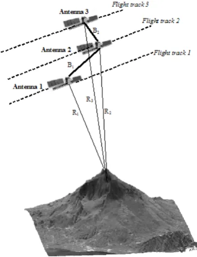
[image:2.595.74.277.446.710.2]

Let us consider a multi-baseline interferometric SAR system (see Fig. 1 for the case of two baselines B1 and B2).

Figure 1. Two-baselines InSAR system geometry

Assuming a discrete ground coordinate system, let Yl(n,m),

with n=1,...,N and m=1,...,M, be the complex envelope of the

image signal of a ground region at the discrete image pixel (n,m), acquired by the l-th antenna:

( )

( )

( )

,...,M m ,...,N n ,...,L, l

(n,m) v e

n,m X e

a(n,m) n,m

Yl j a(n, m) l jαlhn, m l

1 , 1 1

= = =

+

= j ₍₁₎

where L is the number of the interferometric images, N×M is the images dimension, a(n,m) and φa(n,m) are the amplitude

and phase of the radar reflectivity in the (n,m)-th image pixel, Xl(n,m) is the complex envelope of the multiplicative speckle

noise, vl is additive thermal noise, h(n,m) denotes the height

value at the image pixel (n,m), and

α

_l is given by [19]:

θ

λ

π

α

sin

4

0

R

B

_l

l

=

⊥

(2)

where λ is the wavelength, B⊥l is the orthogonal baseline

between the l-th antenna and the reference antenna (master antenna), measured along the direction orthogonal to the range direction, θ is the view angle, c is the speed of light, and R0 is the distance between the master antenna and the center of the scene.

Note that the channel diversity depends on the change of l

α

with the orthogonal baseline.

The problem consists in estimating the height values h(n,m) starting from the L complex SAR images Yl(n,m),

taking into account that the speckle free reflectivity amplitude a(n,m) is also unknown.

Since we consider each image pixel independently from the others, in (1) the dependence on the pixel coordinates can be understood, and in each pixel we can define the data (complex valued) random vector Y=[Y1,Y2,…YL]T and the

speckle (complex valued) random vector X=[X1,X2,… ,XL]T,

where the T denotes the transpose. Moreover, since after SAR image focusing the signal to thermal noise ratio is tipically sufficiently high [20], in (1) we can neglect the additive thermal noise vl. Then, (1) can be rewritten in a

vector form as:

ΦX

Y

₌

_ae

jja ₍₃₎

where

Φ

is

L

×

L

-dimensional diagonal matrix defined as:

[

e

jαh

,

e

jα h

e

jαLh

]

diag

1 2

,

...,

=

Φ

(4)

In (2) a, ja and Φ are deterministic, while in the

assumption of fully developed speckle [18], the complex elements of the speckle vector X have real and imaginary parts which are zero mean mutually uncorrelated Gaussian variables, with variance 2/π (this is a normalization required for obtaining a unit average speckle intensity). Then, X can be modeled as a proper (or circularly symmetric) complex Gaussian random vector [21] with zero mean and covariance matrix CX of size L×L, whose generic element of index (p,q)

is given by:

[

]

_π

4

pq q p

Xpq

E

X

X

γ

where E[·] denotes the expectation operation and γpq is the

coherence between the complex elements

X

_p and

X

_q of the vector X, Note that in the considered assumptions, it is easy to show thar the coherence γpq assumes real values.

The probability density function (pdf) of the vector

X

can, then, be written as:

( )

(

x

C

x

)

C

x

_X

X

X

=

_L

1

exp

-

H -1

f

π

(6)

where x=[x1, x2, …… ,xL]T, the symbol

⋅

denotes the

determinant and

x

H the Hermitian of the vector x.

From (3) we observe that the data vector Y is related to the speckle vector X by a linear relationship. Then Y is still an L-dimensional proper complex Gaussian random vector with zero mean and covariance matrix CY , whose generic

element of index (p,q) is given by:

[ ]

jα h

Xpq q

p

Ypq

E

Y

Y

a

c

e

pq

c

₌

∗

₌

2

(7) where αpq=αp-αq.

From (7), we note that

C

_Y depends on a and h, but does

not depend on the phase φa.

The pdf of the vector Y is, then, given by:

( )

(

y

C

y

)

C

y

_Y

Y

Y

=

_L

1

exp

-

H -1

f

π

(8)

with y=[y1, y2, …… ,yL]T

Now, exploiting (7), we can write:

H

a

Φ

C

Φ

C

_Y

₌

2

_{X (9)} Note that the matrix

Φ

C

_X

Φ

H depends only on h and it is not dependent on the amplitude a.

Exploiting the determinant properties [22], we can write:

X X

Y

Φ

C

Φ

C

C

∏

=

=

=

L k h jα L H

L

_a

_e

k

a

1 2 2

X C =

∏

= -L k h jαk e 1 (10)

Substituting Eqs. (9) and (10) in (8), and considering that

Φ-1_{= Φ}Η_{, we get:}

( )

=

_



_y

_ΦC

-

_Φ

_y

_



C

y

_X

X

Y L

_a

L

_a

H H

f

1 2 2

1

-exp

1

π

(11)

3. Maximum Likelihood Estimation of

Height Profile and Reflectivity

Amplitude

Since the pdf (11) depends only on the parameters a and h, the reflectivity phase value φa cannot be estimated from the

interferometric images and it does not influence the ML estimation of the parameters a and h.

The ML estimate of a and h can be obtained by maximizing the log-likelihood function, obtained by substituting in (11) the measured complex radar images

y

:

(

)

(

)

y

ΦC

Φ

y

C

y

X

X

Y

;a,h

L

_a

L

_a

H H

f

1 2 2

1

-1

log

log

-















=

π

(12) The ML solution for h and a is then given by:

[ ]

a

,

h

(

f

(

;a,h

)

)

a,h

max

log

Y

y

arg

ˆ

ˆ

=

₍₁₃₎

Note that the log-likelihood function (12) will exhibit an unique maximum respect to a, while it presents many local maxima respect to the parameter h, since h appears in the exponent of the complex exponential terms in (4), each of which is periodic with a period depending on the baseline value. Larger periods correspond to smaller baselines. Then, (12) it will be periodic respect to h with a period equal to the least common multiple of the periods of each exponential term. If the least common multiple of these periods is outside the interval range of the admissible height values for the observed scene, or if at least two baselines are in irrational ratio, the likelihood function will exhibit an unique global maximum in the search interval. Anyway, several local maxima will be present, so that a global maximization procedure will be required to find the solution of (13) respect to h.

To show that we can solve (13) in two separate steps, first searching the solution for h and then for a, we compute the derivative of (12) with respect to h and a, and equate it to zero.

Let us consider first the derivative of (12) with respect to h. Since the first term in (12) is independent from h, we have:

(

)

(

)

(

y

)

₍

_y

_ΦC

_Φ

_y

₎

X

Y H H

h

a

h

;a,h

f

1 2

1

log

-∂

∂

-=

∂

∂

(14) Therefore, the ML estimate for h is the value

h

ˆ

satisfying the following nonlinear equation:

(

1

)

₌

0

∂

∂

_y

_ΦC

-

_Φ

_y

X H

H

h

(15)

Since, as stated before, the matrix

_ΦC

_Φ

H

X1

- _{does not}

depend on a, the values of the maxima of (13) respect to h can be found independently on the estimate of the reflectivity amplitude a, using (15) or, equivalently, through the minimization procedure:

y

Φ

ΦC

y

H X H

h

h

ˆ

₌

_arg

_min

-1

part of the Earth surface computed by the interferometric data acquired by the SRTM C-Band SAR system [23] and free distributed by NASA [24].

As far as the estimate of a is concerned, with simple computations, we get:

(

)

(

)

(

log ,h

)

2 2 1

3y ΦC Φ y

y

X

Y H H

a a

L a

a

f _{=- +}

-∂

∂ ; ₍₁₇₎

The ML solution for a is the value

a

ˆ

which equals to zero the expression (17) and is given by:

ˆ

1

L

a

₌

y

H

ΦC

X-

Φ

H

y

₍₁₈₎

From (18), we note that the ML solution

a

ˆ

for a depends on the height value h, through the matrix

Φ

, and it is expressed in closed form. In particular in (18) amounts to perform the square root of the average intensity of the data are obtained after whitening the phase corrected images, in this way the phase coherence is restored by compensating the phase terms introduced by the height profile and the data obtained are decorrelated.

4. Numerical Results

The proposed technique has been tested on synthetic data, which have been simulated using the Envisat-ASAR parameters given in Table 2. Four different sets of three, six, nine and fifteen interferometric images, of size 500×500 pixels, have been simulated following the model given by (3) and using the orthogonal baseline values given in Table 2.

The multiplicative (complex) speckle vector X in (3), for each image pixel, has been generated as a realization of a proper complex Gaussian random vector with zero mean and covariance matrix CX, whose generic elements

c

Xpq, given

by (5), change with the baselines according to the speckle decorrelation model [25]:

π

ϑ

λ

γ

4

tan

1

0

0













∆

-=

⊥

f

R

B

c

c

_Xpq pq (19)

where

B

⊥pq

=

B

⊥p

-

B

⊥q, γ0 is the coherence related to atmospheric conditions and to the thermal noise, c is the propagation velocity and ∆f is the transmitted signal bandwidth. Note that the baseline value

c

f

R

B

_c

₌

λ

0

∆

tan

ϑ

⊥ (20)

[image:4.595.312.553.89.442.2]

corresponds to the complete decorrelation of the interferometric images (γ=0), and in this case the two interferometric images cannot be used to form the phase interferogram. Such baseline is usually referred as the critical baseline. Note that the baselines of Table 2 are all smaller than the critical baseline, which in the case considered is B_⊥c=1081 m.

Table 1. Envisat-ASAR Parameters

Wavelength λ 0.0566 m

View angle θ 23°

Range distance R0 850 km

Pulse bandwidth Δf 16 MHz

Table 2. Orthogonal baselines values

Sensor _Baselines Three _Baselines Six _Baselines Nine _Baselines Fifteen

0 0 0 0 0

1 331 331 331 331

2 541 437 437 379

3 541 491 437

4 747 541 491

5 920 631 523

6 747 541

7 841 583

8 920 631

9 691

10 747

11 781

12 841

13 873

14 920

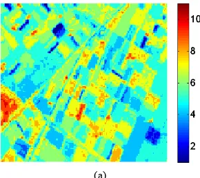
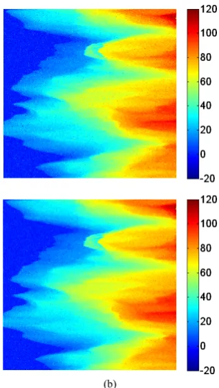
In Figs. 2(a) and 2(b) the amplitude of the radar reflectivity map and the height profile (measured in meters) used to simulate SAR images are shown. Fig. 2(c), instead, shows the inaccurate a priori DEM exploited in the estimation, exhibiting an height error with maximum values of

±

20

m

respect to the true DEM, and with a standard deviation of 3.5 m. Note that the height error values producing a phase of π/4 in correspondence of the minimum and maximum baselines are 3.5 m and 1.2 m, respectively. Then, height error error values between 1.2 m and 3.5 m produce a not negligible unknown phase factor at least in one of the images considered, while height error values larger than 3.5 m produce an unknown phase factor in all images of the considered set.

[image:4.595.359.504.620.749.2]

(b)

[image:5.595.102.255.74.357.2]

(c)

Figure 2. (a) Amplitude of the radar reflectivity of the simulated scene; (b) height profile of the simulated scene; (c) a priori inaccurate height profile of the simulated scene exploited in the estimation procedure.

Since the height estimate is independent on the value of the reflectivity amplitude a, as shown in the previous Section, we can first estimate h using (16). Note that in (16) the knowledge of the speckle covariance matrix CX is required.

As it is usually done in interferometic applications, it has been estimated from the data by using a sliding window whose dimensions have to be small enough to assume that the reflectivity amplitude and the height values in the window pixels are constant, and large enough to have a sufficiently accurate estimate of the statistical average [25]. The size generally adopted is 5×5 pixels. Moreover, we note that when the number of baselines increases and the baselines assume values which are close each other, the matrix CX becomes ill conditioned, and special care has to

be devoted to its inversion, which can be performed by uding singular value decomposition (svd) [22].

The height estimation accuracy can be evaluated by computing the root mean square error (RMSEh). We remind

that the RMSEh is the result of two contributions: statistical

errors due to the presence of noise, and errors due to solution ambiguity [10]. The latter contribution can be minimized by restricting the solution search interval around the height values of the low resolution inaccurate a priori DEM, which for instance cam be provided by SRTM-DEMs [24]. In such case, the RMSEh can be assumed dependent only from the

phase noise, and can be consistently compared with the square root of the Cramer Rao Lower Bound for h (CRLBh),

which represents the maximum accuracy attainable with an efficient estimator [26] and it does not take into account the possible occurrence of ambiguous solutions. Then, to reduce

the occurrence of ambiguous solutions,we search for the ML solution in an interval 40 m wide around the a priori height profile of the scene.

Table 3. Height estimation accuracy RMSEh

Eq. (16) only phase dataRMSEh CRLBh1/2

3 images 5.77 5.95 2.01

6 images 3.61 5.29 1.40

9 images 3.05 4.93 1.37

15 images 2.77 4.90 1.34

The RMSEh values in case of three, six, nine and fifteen

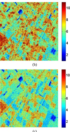
images are presented in Table 3, while the height reconstruction obtained from six images and fifteen images are shown in Figs. 3(a) and 3(b) respectively. Table 3 also shows the square root of CRLBh, to assess the maximum

accuracy that can be achieved by processing the considered data sets. As expected, RMSEh decreases and approaches the

corresponding CRLBh1/2 values when the number of images

increases. The better quality of the height profile obtained with 15 baselines is evident also in Fig. 3.

(b)

Figure 3. Height reconstruction obtained through Eq. (16) using: (a) 6 images and (b) 15-images

[image:5.595.313.552.121.213.2] [image:5.595.352.511.336.617.2]

multi-baselines interferograms [10], since the spectra of the different images are overlapping each other. The adoption of this approximation is as more critical as more the number of baselines increases, since in this case the image spectra overlapping becomes more relevant.

Fig. 4 shows the results obtained from only phase data in the case of six and fifteen images and it shows a worse quality respect to the reconstruction of Fig. 3. The RMSEh

values are presented in Table 3. It is noted that the estimation exploiting only phase data exhibits a worst performance. The difference in performance becomes more evident when the number of images increases, since the adopted approximation of statistical independence among the multiple phase interferograms becomes more critical when the baselines step up within the critical baseline extent.

(a)

(b)

Figure 4. Height reconstruction from only phase data using (a) 6 images and (b) 15 images

As far as the estimation of the amplitude reflectivity a is concerned, it can be evaluated using (18). Note that the estimate (18) depends on h through the matrixΦ=Φ(h) (see (4)) and on the speckle covariance matrix CX. To analyze the

influence of h and of the mutual correlation of the multi-baseline images on the estimation of a , we can consider the following three cases:

1) Incoherent interferometric multi-look (IML): The matrix CX is approximated with

C

_X=

I

_L, with

I

_L

the L-dimensional identity matrix, then also

H

Φ C

Φ X =

I

L . This assumption corresponds to

uncorrelated images. In this case (18) becomes:

1

ˆ

1 2

∑

=

=

L

k k

IML

_L

y

a

(21)

Eq. (21) amounts to perform the incoherent average of the intensity images.

2) Partially coherent interferometric multi-look (PCML): The matrix is approximated with

Φ

ˆ

=

Φ

( )

h

₀ , where h0 is the a priori inaccurate DEM. This amounts to use a

rough approximation of the phase factors introduced by the height profile. The image correlation, instead, is taken into account through the matrix

C

_X. In this case (18) becomes:

( )

( )

ˆ 0 1 0

L h h

aPCML yHΦ CXΦH y

-= (22)

Eq. (22) amounts to perform the average of the intensities of the images obtained after whitening and phase compensating the L measured images for the available a priori DEM h0. Note that phase compensation partially

restores the phase coherence, while the whitening operation uncorrelates the data.

3) Fully coherent interferometric multi-look (FCML): in this case the matrix Φ=Φ(h) is approximated with

( )

h

ˆ

ˆ

_Φ

Φ

=

, where

_h

ˆ

is the estimated height value. In this case (18) becomes:

( )

ˆ

( )

ˆ

ˆ 1

L h h

a_FCML= yHΦ CX-ΦH y ₍₂₃₎

Eq. (23) amounts to perform the average of the intensities of the images obtained after whitening and phase compensating the L measured images using the estimated height profile. Note that in this case phase compensation produces an higher phase coherence, since the used height values are more accurate, while whitening uncorrelated the data.

Figs. 5, and 6 show the IML, the PCML and the FCML reconstructed image amplitudes, in the case of six and fifteen images, respectively. As expected, comparing by a visual inspection Figs. 5 and 6 with Fig. 2(a), it is quite evident that FCML outperforms the other methods.

[image:6.595.358.504.605.740.2]

(b)

[image:7.595.104.252.73.352.2]

(c)

Figure 5. Amplitude estimation from 6-images: (a) IML, (b) PCML, (c) FCML

Two different parameters are evaluated to quantitatively analyse the estimation accuracy of a: the normalized root mean square value of the estimation error (NRMSEa),

defined as:

    

  

     

-= ˆ 2

NRMSE

a a a E

a (24)

where a is the true amplitude reflectivity value and

a

ˆ

is its estimated value, and the equivalent numbers of looks (ENL), defined as:.

[ ]

[ ]

(

)

[

2

]

2

) ( ENL

p E p E

p E p

-= =

[ ]

_{[ ]}

p Var

p

E 2

(25) where Var [·] denotes the variance, p is the intensity (square amplitude) to be tested (

_ˆ

2

IML

a

,

a

ˆ

_PCML2 ,

a

ˆ

_FCML2 ) and the statistical averages are evaluated through sample extended to homogeneous areas over the image.

For a single image, the ENL is about equal to one, since the variance and the square statistical average assumes the same value. Note that the higher the ENL, the better is the speckle reduction and, then, the capability of distinguishing different intensity levels.

(a)

(b)

[image:7.595.357.508.74.501.2]

(c)

Figure 6. Amplitude estimation from 15-images: (a) IML, (b) PCML, (c) FCML

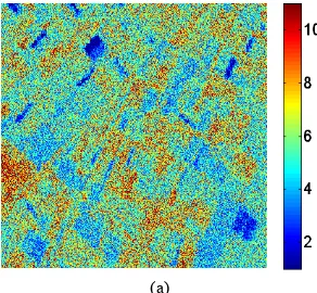
The values of the parameters defined above, evaluated on the amplitude images obtained starting from three, six, nine and fifteen images, are shown in Table 4.

Table 4. Reflectivity amplitude estimation accuracy parameters

NRMSEa

IML NRMSEPCML a

NRMSE

a

FCML CRLBa

1/2 ENL

on IML image on PCML image ENL on FCML image ENL

3 images 0.415 0.495 0.322 0.22 1.47 1.37 2.17

6 images 0.382 0.473 0.251 0.14 2.05 4.07 4.98

9 images 0.394 0.425 0.231 0.11 1.40 3.41 8.01

15 images 0.401 0.315 0.183 0.08 1.49 7.55 11.95

The results in Table 4 show that when the number of images increases, performance of FCML becomes noticeably better than IML because the effect of the mutual correlation between the images becomes more significant. In fact, we note that, due to the data correlation, the intensity average performed by IML produces only a small effect for the speckle reduction on the reflectivity amplitude, which does not increases when the number of the images increases. Moreover, comparing the accuracy parameters obtained with PCML and FCML processing, we observe that the effect of the improvement of the height profile accuracy is always evident and it increases when the number of the images increases.

Table 4 also shows the corresponding square root of the CRLB for a, to assess the maximum accuracy achievable from the considered data sets.

5. Conclusions

In this paper we presented a method to improve the DEM estimation accuracy, starting from correlated multi-baseline interferometric images and a low resolution inaccurate a priori DEM of the observed scene. The method takes into account the correlation among all the interferometric images. This is very important, since multi-baseline acquisitions are almost always mutually correlated. The method exploits both amplitude and phase of the interferometric data and it is based on an ML estimation technique. It allows to estimate both the height profile and the speckle reduced reflectivity intensity. It has been shown that the estimation procedure can be split in two steps: first the height estimation is performed independently from the reflectivity amplitude, then the speckle reduced reflectivity amplitude is evaluated taking into account both the images correlation and the phase factors introduced by the height profile.

Numerical results on simulated data show that the obtained height estimation accuracy is better than that achievable with the methods exploiting only phase data, which adopt the approximation of statistical independence of the phase interferograms, due to the difficulty of expressing their “exact” likelihood function in closed form. Performance improvement is as larger as the number of baselines considered becomes higher. Moreover, as expected, it is shown that the height accuracy improves with the number L of the processed images with a low slower than the linear one, due to the images correlation.

As far as the estimation of the reflectivity amplitude is

concerned, numerical experiments show that both the image correlation and the phase factors introduced by the height profile of the observed scene have to be considered. In particular, it is shown that the exploitation of the improved accuracy height estimation obtained in the first step, allows to a noticeably improvement of the reflectivity amplitude quality.

REFERENCES

D. Massonet, K. L. Feigl, “Radar interferometry and its [1]

application to changes in the earth’s surface,” Rev. Geophys., vol. 36, pp. 441–500, 1998.

J. O. Hagberg, L. M. H. Ulander, “On the optimization on [2]

interferometric SAR for topographic mapping,” IEEE Trans. Geosci. Remote Sensing, vol. 31, pp. 303–306, Jan. 1993. F. K. LI, R. M. Goldstein, “Studies of multibaseline [3]

spaceborne interferometric synthetic aperture radar”, IEEE Trans. Geosci. Remote Sensing, vol. 28, pp. 88–97, Jan. 1990. A. Ferretti, C. Prati, F. Rocca, “Multibaseline DEM [4]

Reconstruction: the Wavelet Approach”, IEEE Trans. Geosci. Reote. Sensing, vol. 37, pp. 705-715, March 1999.

G. Fornaro, V. Pascazio, G. Schirinzi, “Resolution [5]

improvement via multipass SAR imaging,” in Proc. IGARSS, Sydney, Australia, Jul. 2001, pp. 2734–2736.

S. Guillaso, A. Reigber, L. Ferro-Famil, E. Pottier, “Range [6]

Resolution Improvement of Airborne SAR Images”, IEEE Geosci. Remote Sensing Letters, vol. 3, pp. 135–139, Jan. 2006

A. Reigber, A. Moreira, “First demonstration of airborne [7]

SAR tomography using multibaseline L-band data”, IEEE Trans. Geosci. Remote Sensing, vol. 38, pp. 2142-2153, Sept. 2000.

G. Fornaro, F. Serafino, “Imaging of Single and Double [8]

Scatterers in Urban Areas via SAR Tomography”, IEEE Trans. Geosci. Remote Sensing, vol. 44, pp. 3497 - 3505, Dec. 2006.

Pascazio V., Schirinzi G., “Estimation of Terrain Elevation [9]

by Multi-Frequency Interferometric Wide Band SAR Data”, IEEE Signal Processing Letters, vol. 8, pp. 7-9, 2001. V. Pascazio, G. Schirinzi, “Multi-Frequency InSAR Height [10]

Reconstruction through Maximum Likelihood Estimation of Local Planes Parameters”, IEEE Trans. Image Proc., vol. 11, pp. 1478-1489, Dec. 2002.

Posteriori Estimation of Height Profiles in InSAR Imaging”, IEEEGeosci. Rem. Sensing Letters, vol. 1, pp. 66-70, 2004. M. Eineder, N. Adam, “A Maximum-Likelihood Estimator to [12]

Simultaneously Unwrap, Geocode, and Fuse SAR Interferograms from Different Viewing Geometries into One Digital Elevation Model”, IEEE Trans. on Geosci. Remote Sens., vol 43, pp. 24–36, 2005.

G. Fornaro, A. Monti Guarnieri, A. Pauciullo F. De-Zan, [13]

“Maximum likelihood multi-baseline SAR interferometry”, IEE Proc.-Radar Sonar Navig., Vol. 153, pp. 279-288, 2006.

G. Franceschetti, M. Migliaccio, D. Riccio, G. Schirinzi, [14]

"SARAS: a SAR (Synthetic Aperture Radar) Raw Signal Simulator'', IEEE Trans. Geosci. Remote Sensing, vol. 30, pp. 110-123, 1992.

O. Loffeld, H. Nies, S. Knedlik, Yu Wang, “ Phase [15]

Unwrapping for SAR Interferometry—A Data Fusion Approach by Kalman Filtering”, IEEE Trans. on Geosci. Remote Sens., vol. 46, pp. 47-58, 2008.

C. Tison, F. Tupin, H. Maitre, “A Fusion Scheme for Joint [16]

Retrieval of Urban Height Map and Classification From High-Resolution Interferometric SAR Images”, IEEE Trans. on Geosci. Remote Sens., vol. 45, pp. 496-505, 2007.

M. Lucido, F. Meglio, V. Pascazio, G. Schirinzi, [17]

“Dual-Baseline SAR Interferometry from Correlated Phase Signals”, IEEE Radar Conf. 2008, pp. 2071-2076, Roma, May 2008.

J. Goodman, "Statistical Properties of Laser Speckle [18]

Patterns," in Speckle and Related Phenomena, 2nd Edition, J. C. Dainty Ed., Springer Verlag, NY 1984.

R. Bamler, P. Hartl, “Synthetic Aperture Radar [19]

Interferometry”, Inverse Problems, vol. 14, pp. R1-R54, 1998.

D. Massonet, J. C. Souyris, “Synthetic Aperture Radar [20]

Imaging”, Efpl Press, 2008.

F. D. Neeser, J. L. Massey, “Proper Complex Random [21]

Processes with Applications to Information Theory ”, IEEE Transactions on Information Theory, vol. 39, pp. 1293-1302, July 1993.

G. H. Golub, C. F. Van Loan, Matrix Computations, 3rd _ed., [22]

Johns Hopkins, 1996.

P. A. Rosen, S. Hensley, E. Gurrola, F. Rogez, S. Chan, J. [23]

Martin, E. Rodriguez, “SRTM C-Band Topographic Data Quality Assessments and Calibration Activities”, in Proc. IGARSS‘01, pp. 739–741, Sydney (AUS), 2001.

http://edc.usgs.gov/products/elevation.html (accessed in Dec. [24]

2008).

H. A. Zebker, J. Villasenor, “Decorrelation in Interferometric [25]

Radar Echoes”, IEEE Trans. on Geosci. Remote Sens., vol. 30, pp. 950-959, 1992.

S. M. Kay, Fundamentals of Statistical Signal Processing: [26]