Helmholtz Manakov solitons

Helmholtz­Manakov solitons

Christian, JM, McDonald, GS and Chamorro­Posada, P

http://dx.doi.org/10.1103/PhysRevE.74.066612

Title Helmholtz­Manakov solitons

Authors Christian, JM, McDonald, GS and Chamorro­Posada, P

Type Article

URL This version is available at: http://usir.salford.ac.uk/id/eprint/298/ Published Date 2006

USIR is a digital collection of the research output of the University of Salford. Where copyright  permits, full text material held in the repository is made freely available online and can be read,  downloaded and copied for non­commercial private study or research purposes. Please check the  manuscript for any further copyright restrictions.

Helmholtz-Manakov solitons

J. M. Christian, G. S. McDonald and P. Chamorro-Posada †

Joule Physics Laboratory, School of Computing, Science and Engineering,

Institute for Materials Research, University of Salford, Salford M5 4WT, U.K.

†_{Departmento de Teoría de la Señal y Comunicaciones e Ingeniería Telemática,}

Universidad de Valladolid, ETSI Telecomunicación, Campus Miguel Delibes s/n,

47011 Valladolid, Spain.

Accepted in Physical Review E, 21st September 2006

ABSTRACT

A novel spatial soliton-bearing wave equation is introduced, the Helmholtz-Manakov

(H-M) equation, for describing the evolution of broad multi-component self-trapped

beams in Kerr-type media. By omitting the slowly-varying envelope approximation,

the H-M equation can describe accurately vector solitons propagating and interacting

at arbitrarily large angles with respect to the reference direction. The H-M equation

is solved using Hirota’s method, yielding four new classes of Helmholtz soliton that

are vector generalizations of their scalar counterparts. General and particular forms

of the three invariants of the H-M system are also reported.

PACS numbers: 42.65.Tg (optical solitons), 42.79.Ta (optical computers),

I. INTRODUCTION

Vector solitons are well known in Optics [1,2]. They are multi-component,

localized structures that can become dominant modes of a system when linear

broad-ening effects are offset by non-linearity. During pulse propagation, on the one hand,

vector solitons can arise when dispersion is balanced by self- and cross-phase

modula-tion. Spatial soliton beams, on the other, can result if diffractive spreading is opposed

by medium self- and mutual-focusing. Many years ago, Manakov [3] proposed a

vec-tor extension of the scalar Non-Linear Schrödinger (NLS) equation [4] to describe

multi-component pulse/beam evolution in the presence of positive Kerr non-linearity.

Using inverse-scattering theory, he was able to derive an exact analytical

2-component sech-type soliton solution.

In birefringent optical fibres, vector solitons play a central role in describing

polarization-division multiplexing (PDM) configurations, where light coupled into the

fibre is polarized along two transverse orthogonal axes [5]. Over sufficiently long

distances, birefringence can average out stochastically to zero, and the model

captur-ing evolution is the (temporal) Manakov equation [6]. In spatial contexts,

multi-component solutions for a defocusing (negative) Kerr non-linearity have been

re-ported [7]. These new solutions have a more complicated (topological) structure than

their more familiar sech-type counterparts in the focusing regime [3]. Manakov-like

solitons, comprising two orthogonal transverse field components, have been observed

in birefringent Kerr-type planar waveguides [8]. Multi-component spatial solitons in

( )2

χ [9] and χ( )3 -like [10] photorefractive media have also received attention, and

new types of structures such as multi-hump [11] and holographic [12] solitons have

Recently, it has been shown that collisions between Manakov solitons are

ine-lastic, and that there is a redistribution of energy between the interacting components

[13]. Such an intrinsic effect has no analogue in scalar (i.e. NLS) theory, where the

energy and momentum of each constituent soliton is preserved [4]. It has been

sug-gested [14] that this unique property of the Manakov system could provide the basis

for optical computing with solitons [15]. The energy-exchange process was found to

depend critically upon the angle between the interacting beams. It is therefore

desir-able to have a model capdesir-able of capturing arbitrary angles.

The main interest in this Article lies with the oblique propagation of

multi-component spatial solitons in Kerr planar waveguides. In this geometry, there is a

longitudinal (reference) and a single effective transverse dimension that, in uniform

media, are physically equivalent. We propose the novel Helmholtz-Manakov

equa-tion as a 2-component generalizaequa-tion of the scalar Non-Linear Helmholtz (NLH)

equation [16]. This model is appropriate for capturing the propagation [17] and

inter-action [18] of broad vector-soliton beams at arbitrary angles with respect to the

refer-ence direction. Here, we present four new families of exact analytical soliton solution

to the H-M equation, and derive the corresponding conservation laws.

II. HELMHOLTZ NON-PARAXIALITY

The NLH and H-M equations provide a full description of oblique (off-axis)

evolution for broad optical beams of moderate intensity [16-18]. Under these

condi-tions, the polarization-scrambling term in Maxwell’s equations can be neglected

[19-21] and this leads to two important simplifications: (i) in uniform media, the

(ii) the electric field may be regarded as being purely transverse (we can ignore the

longitudinal component). For NLH solitons, one typically considers a TE mode

po-larized in the plane of the waveguide [18]. For vector solitons, the electric field can

have two orthogonal polarization components [3]. In this particular context, the H-M

equation is a valid model when birefrigence can be neglected [22]. Alternatively, the

H-M model can describe the interplay between two incoherently-coupled fields

shar-ing the same polarization state where, typically, both are TE modes [18]. This latter

consideration could be extended to the case of N components [23].

The oblique evolution of broad beams context defines the Helmholtz

non-paraxial scenario [16-18], which is physically and mathematically distinct from the

narrow-beam regime considered by other authors. Perturbative narrow-beam

correc-tions to the governing equation [19-21,24], derived from single-parameter

order-of-magnitude analyses of Maxwell’s equations, are both unnecessary (we consider only

broad beams) and invalid (off-axis effects are not quantified solely by a single small

parameter) in Helmholtz non-paraxality. The accurate description of

obliquely-propagating and interacting beams, relative to the reference direction, requires one to

respect the equivalence of the transverse and longitudinal dimensions in uniform

me-dia. This is achieved by avoiding the slowly-varying envelope approximation

(SVEA); NLH and H-M models then arise as natural governing equations [17,18].

In a normalized form, the H-M equation is given by

( )

2 2

†

2 2

1 2 i

κ

ζ

ζ ξ

∂ ₊ ∂ ₊ ∂ _{± =}

∂

∂ ∂

U U U

where the sign flags a focusing (+) or a defocusing (–) Kerr non-linearity. ±

0 2x w

ξ = and ζ =z L_D

0 w

are the scaled transverse and longitudinal coordinates,

normalized to the waist and diffraction length 2 0 2

D

L =kw of a reference

Gaus-sian beam, respectively. The column vector is the dimensionless electric field in U

( )

( )

(

)

E U , where k=2πn0 λ, λ is the optical wavelength, is

the linear refractive index at the optical frequency,

0 n

(

)

0 0 2 D

E = n k n L and is the

Kerr coefficient.

2

n

(

) (

)

1

= =

]

2 _{2 2}

0 λ w0 4π n0

kw

κ is the inverse beam-width

parame-ter. In the case of two field components, one has that U , where T denotes

the transpose, and is the Hermitian adjoint of U. A further generalization to N

components then involves including further entries in .

[

†

U

U

The restoration of spatial symmetry in the governing equation [17] leads to

several novel features absent from paraxial theory. Firstly, there is no physical

dis-tinction between transverse (x) and longitudinal (z) coordinates and light is allowed to

diffract in both these dimensions. Secondly, inclusion of κ∂_ζζ leads to a dispersion

relation that supports both travelling- and standing-wave solutions [18]. This is in

contrast to the NLS [4] and Manakov [3] equations, where the SVEA breaks the

symmetry between not only x and z, but also between +z and –z, (backward-travelling

waves are not supported). Thus, paraxial wave equations are subjected to the physical

limitation of describing beams that are either axial or very nearly axial.

The inherent bi-directionality of NLH-based models leads to angular beam

same beam from different frames of reference, and is a requirement based on

geome-try [16]. The Helmholtz non-paraxial formalism also allows for a well-defined

con-nection between the soliton velocity V in the

(

)

θ (relative to the z axis) in the unscaled

( )

tanθ = 2κV. (2)

Equation (2) verifies that the (purely geometrical) Helmholtz correction may

assume an arbitrarily large value, even for beams with

2 2κV

0

κ . During off-axis

evolu-tion, one can have a regime where _2κV2 _~O

( )

because the beam is always broad. This possibility demonstrates that

de-scriptions based solely upon -type expansions of Maxwell’s equations are

inappro-priate for capturing the angular type of non-paraxiality [19-21,24]. Indeed, the

domi-nant Helmholtz correction to paraxial theory, embodied in Eq. (2), is determined

solely by the beam’s propagation angle and can be of any order irrespective of the size

of .

1

( )

κ

κ

κ

III. HELMHOLTZ-MANAKOV SOLITONS

A. Solitons in self-focusing Kerr media

For a focusing Kerr medium, the simplest case to consider is that of a vector

beam with two forward-propagating constituent components, each with a symmetric

sech-type profile. The most straightforward method of obtaining such solutions is to

use an ansatz approach to seek the on-axis solution, and then apply a rotational

trans-formation [25] to seek the more general off-axis beam. The resulting bright-bright

(

)

(

)

2

2 2

1 2

, sech exp exp ,

2 2 1 2 1 2 V i V V V

η ξ ζ

i

κη ζ

ξ ζ η ξ ζ

κ κ κ κ    +  _ +  _  =   _− + _{ } +       +     

U C − _

 (3a)

where,

( )

( )

C . (3b)

C is a complex column vector obeying C C† =1, while η defines the amplitude and

the transverse velocity. The free parameter

V α determines the strength of the

exci-tation in each component, and δ_j ( j=1, 2) are the component phases. The choice of

values of α and the δ_j’s allows a wide variety of soliton states to be constructed.

The second class of vector beam that a focusing Kerr medium can support is

the bright-dark soliton, for which the forward-propagating solution is

(

)

(

)

(

)

2 2 2

0 ₂

2 2

2

, cos sech

1 2

1 2 2

exp exp ,

1 2 2 2

a W

A B a

W

a

i W

W

ξ ζ

ξ ζ φ

κ

κ χ _{ζ ζ}

ξ i

κ κ κ

 +  = + _{ } +    _{+ +  } _   × _− + _{ }  +       − _  (4a)

(

)

(

)

2 2

, cos tanh sin

1 2

1 4

exp exp ,

1 2 2 2

a W

B B i

W

i V i

V

ξ ζ

ξ ζ φ φ

κ

κχ _ξ ζ ζ

κ κ κ

  +   = _{  }+ _ +        _{+  } _ ×  _− + _ _ +         − _  (4b)

This structure comprises a Helmholtz bright soliton [25] in one component, and a

dark-type topological excitation in the other. The tanh component (4b) is generally

grey, and has an intrinsic velocity,

(

)

0 _{2 2 2}

tan

1 2 2 tan

a V

a

φ

κ χ φ

=

This velocity depends upon both the non-paraxial parameter κ and the plane-wave

background intensity χ2 ≡B₀2. When , the dark component is null and one

recovers the Helmholtz Kerr scalar bright soliton [25]. The net velocity W of the

vec-tor beam (4) is then given by

0 0 B → 0 0 1 2 V V VV κ

W = −

+ . (6)

As in the case of the scalar Helmholtz dark soliton [26], W has the physical

interpreta-tion of velocity summainterpreta-tion in the unscaled reference frame.

B. Solitons in defocusing Kerr media

When seeking a general dark soliton of the defocusing NLH equation [26], an

ansatz approach cannot determine the full solution (geometrical considerations also

have be to made). Similar difficulties arise in the vector case. Thus, Hirota’s method

[27] has been used to solve the defocusing H-M equation. The forward-propagating

dark-bright vector soliton solution is given by

(

)

(

)

2 2

, cos tanh sin

1 2

1 4

exp exp ,

2 2

1 2

a W

A A i

W

i V

W

ξ ζ

ξ ζ φ φ

κ

κχ _ξ ζ ζ

i κ κ κ   +   =  _ _+    +      _{−  } _   × _− + _{ } +         − _  (7a)

(

)

(

)

(

)

2 2 2

0 ₂

2 2

2

, cos sech

1 2

1 2 2

exp exp .

1 2 2 2

a W

B A a

W a

i W

W

ξ ζ

ξ ζ φ

κ

κ χ

i

ζ ζ

ξ

κ κ κ

 +  = − _{ } +    _{+ −}       × _− + _{ }  +       − _  (7b)

The grey component (7a) has an intrinsic velocity

(

)

0 _{1 2}

2 2 2

tan

1 2 2 tan

a

a

V φ

κ χ φ

=

 _{− +} 

 

where , and the net velocity W is given by Eq. (6). The dark-bright soliton is

constrained by the condition . When the equality is satisfied, the bright

component vanishes and the remaining component (i.e., the primary component)

re-covers an exact non-paraxial dark soliton [26]. 2

0 A

χ≡

2 2

0 cos

A φ ≥_a2

The bright-dark and dark-bright solutions are characterized by three velocities,

V, V₀ and W, which are associated with the propagation angles tanθ = 2κV ,

0 0

tanθ = 2κV and tan

(

)

κ

[20] (note that any two velocities can be

chosen independently). However, it is important to note that these solutions are not

equivalent. When the dark components have the same parameters (i.e. background

intensities and values of , a and φ), the soliton intensity profiles different slightly

from one another due to their different intrinsic velocities, given by Eqs. (5) and (8),

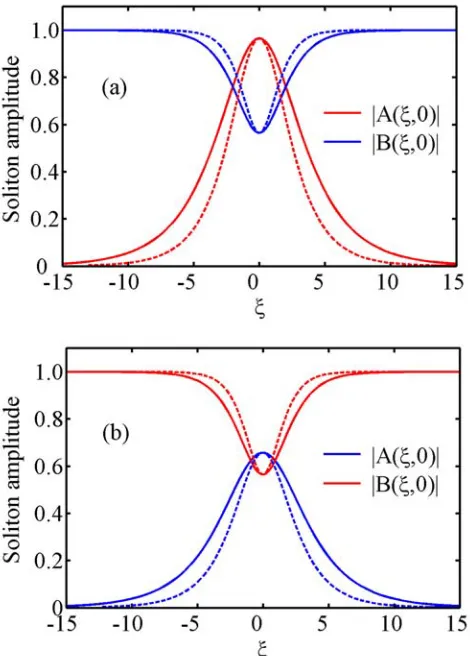
respectively (see Fig. 1). Another distinction between dark-bright and bright-dark

so-lutions is that the primary component (that which can propagate stably when the other

component is not excited) is a dark soliton in the former, and a bright soliton in the

latter.

The secondary component of these mixed-pair (that is, bright-dark and

dark-bright) beams possesses anti-guiding properties, a phenomenon seen also with

Mana-kov solitons [7]. For the dark-bright soliton, the bright (secondary) component,

propagating in the waveguide induced by the dark (primary) component, has an

inten-sity maximum at its centre. The presence of such a maximum in a defocusing

me-dium leads to a lowering of the refractive index at the beam centre, thus weakening

com-petitive process between the non-linear refractive index changes brought about by the

individual dark and bright components. When these processes are balanced precisely,

an equilibrium state is formed and a vector soliton may propagate. These refractive

index changes are reversed for the bright-dark soliton in a focusing medium, but the

underlying physics remains the same.

The (forward-propagating) dark-dark vector soliton of the defocusing H-M

equation has also been found using Hirota’s method

(

)

(

)

2 1 2 1

, cos tanh sin

1 2

1 4

exp exp ,

2 2

1 2

a W

A A i

W

i V i

V

ξ ζ

ξ ζ φ φ

κ

κχ _ξ ζ ζ

κ κ κ   +   =  _ _+    +      _{−  } _   × _− + _{ } +         − _  (9a)

(

)

(

)

2 2 2 2

, cos tanh sin

1 2

1 4

exp exp ,

2 2

1 2

a W

B B i

W

i V

V

ξ ζ

ξ ζ φ φ

κ

i

κχ _ξ ζ ζ

κ κ κ   +   =  _ _+    +      _{−  } _   × _− + _{ } +         − _  2 0 (9b)

where is the total (incoherent) intensity of the vector beam. The

ex-pressions for the intrinsic velocities are

2 2

0

A B

χ ≡ +

(

)

0 _{1 2}

2 2 2

tan

1 2 2 tan

j j j a a V φ

κ χ φ

=

 _{− +} 

 

, (10)

where j=1, 2, and there is a dependence not only on the non-paraxial parameter κ

but also on _χ2_{. The soliton parameters are connected by the implicit relationship}

that removes a degree of freedom from the system. The

two components necessarily have the same net velocity W, but their plane-wave back-2 2

0 1

A φ B2 2

0 2

grounds may travel in different directions. Note that Eq. (9) for the dark-dark soliton

is formally identical to Eq. (8) for the dark-bright solution.

Paraxial solitons of the NLS [4] and Manakov [3] equations can have

arbitrar-ily large values of phase angle φ π< 2. In contrast, H-M solitons possess a

maxi-mum “greyness” denoted by φmax. For the defocusing non-linearity, φmax is defined

by

2

max 2

1 4 tan

2 a

κχ φ

κ

−

= , (11)

where 2 for the dark-bright soliton, and 0

A

χ ≡ 2 2

0

2 2

0

A B

χ ≡ + in the dark-dark case. A

similar expression can be derived for the bright-dark solution (4). This limit

corre-sponds to a physical constraint on the largest intrinsic velocity that a dark soliton may

possess, depending on the background intensity. When φ →φ_max, the intrinsic

veloc-ity diverges and the dark component propagates in a direction perpendicular to that of

the background plane wave, θ₀ → ±π 2 [26].

IV. CONSERVED QUANTITIES

Knowledge of the invariants is of fundamental importance. They are also

use-ful tools for testing the integrity of any numerical scheme used in computer

simula-tions [28]. The H-M equation (1) may be regarded as the Euler-Lagrange equation of

motion corresponding to a Lagrangian density L, from which one defines a pair of

ca-nonically-conjugate momentum variables, π and π :

(

)

( )

† † † ₂

† † 1 1 †

, ,

2 2

i

L κ

ζ ζ ζ ζ ξ ξ

 ∂ ∂  ∂ ∂ ∂ ∂

= _ − _− − +

∂ ∂ ∂ ∂ ∂ ∂

 

U U U U U U

U U U U U U

2 (12a)

† 2 L i ζ κ ζ   ∂ ∂ ≡ = −_ + _

∂U _ ∂ _U

π , _†

2 L i ζ κ ζ  ∂ ≡ =_ − ∂ ∂U _{ }U

π ∂ _

U

, (12b)

and . It is then straightforward to calculate the conserved quantities [29].

The fundamental quantity is the energy-flow E, which arises from invariance of L

un-der a global phase transformation. The second conserved quantity is the linear

mo-mentum M of the system, found from invariance under an infinitesimal translation in

ζ ≡ ∂ζ

U

ξ. The third conserved quantity is the Hamiltonian H, derived from consideration of

translations in the evolution variable, ζ .

†

† †

E dξ iκ

ζ ζ +∞ −∞   ∂ ∂  =  −  _∂ − _∂      

∫

† † †

† _,

2 i

M dξ κ

ξ ξ ζ ξ ξ ζ

+∞ −∞   ∂ ∂  ∂ ∂ ∂ ∂  = _{ } − _− _ + _ ∂ ∂ ∂ ∂ ∂ ∂       

∫

 (14)

( )

† † ₂

† 1

2 2

H dξ κ

ξ ξ ζ ζ

+∞ −∞  ∂ ∂ ∂ ∂  = _ − − _ ∂ ∂ ∂ ∂  

∫

Equations (13)-(15) also apply to the scalar NLH equation, by allowing one of the

field components to be null. For bright-bright H-M solitons, it is found that:

_{E=2η 1 2+ κη}2 _{, (16a)}

2 2

2 3 4

3 _{1 2}

M V V κη η κ + =

+ , (16b)

2 2 2 3 4 1 2

3 _{1 2}

H

V

η _κη η κη

κ κ _κ

+

= + −

+ . (16c)

These results are exactly the same as for the scalar bright Helmholtz soliton [25]. As

expected they reduce to their paraxial counterparts in the multiple limit ,

and [1,2]. It is interesting to note that

0

κ →

2 ₀

κη → _κV2_{→0 ∂H M V∂ = (as in the}

compo-nent, the invariant integrals (13)-(15) can be strongly divergent. A renormalization

procedure is thus necessary to remove such infinities.

V. CONCLUSION

In this Article, we have considered broad multi-component spatial beams in

uniform planar waveguides, placing particular emphasis on the inherent spatial

sym-metry of such systems. The novel Helmholtz-Manakov equation, which generalizes

our earlier work on scalar beams [16-18,25,26,30], has been introduced and its

2-component solutions (localized, mutually-trapped structures) have been derived using

Hirota’s method. The new solutions uncover explicit physical dependencies of novel

quantitative and qualitative features. In a following publication, we will present the

results of a perturbative analysis, which has tested and verified the stability properties

of each new soliton family.

We expect the H-M equation and its soliton solutions to be relevant in other

optical contexts, such as photorefractives [9,10], multi-hump [11] and holographic

[12] solitons. It is also likely to provide a key analytical platform in the

understand-ing of vector-soliton interactions (both co- and counter-propagatunderstand-ing scenarios) at

arbi-trarily large angles [18]. We expect new doors of investigation to be opened by lifting

the angular restrictions of current paraxial models. This has particular importance, for

example, in the field of optical computing [14,15]; it may also find application in

op-tical contexts involving feedback [31]. Helmholtz generalizations offer broad

physi-cal insight into a wide variety of angular geometries by taking full account of the role

ACKNOWLEDGEMENTS

The authors would like to acknowledge financial support from EPSRC

FIGURE CAPTIONS

FIG. 1 (color on-line). Characteristic angular beam-broadening effects associated

with Helmholtz solitons for (a) bright-dark, and (b) dark-bright cases. Solid line:

( )

A ξ ; dashed line: B

( )

4 10

κ ₌ −

. Dotted lines correspond to paraxial solutions. For a

non-paraxial parameter , a transverse velocity of V ≈70.71 yields a physical

propagation angle θ =45° so that 2κV2=O

( )

0.5 a

1 and one has a strongly non-paraxial

regime. Other solution parameters are = , φ π= 6, B₀ =1 [in (a)] and

[in (b)].

FIGURE 1

J. M. Christian et al.

___________________________________________________________________________________

[1] Y. S. Kivshar, Opt. Quant. Elect. 30, 517 (1998).

[2] Y. S. Kivshar and B. Luther-Davies, Phys. Rep. 298, 81 (1998).

[3] S. V. Manakov, Sov. Phys. JETP 38, 248, (1974).

[4] V. E. Zakharov and A. B. Shabat, Sov. Phys. JETP 34, 62 (1972); 37, 823

(1973).

[5] C. R. Menyuk, J. Opt. Soc. Am. B 5, 392 (1988); IEEE J. Quantum Electron.

QE-23, 174 (1987); Opt. Lett. 12, 614 (1987).

[6] J. Yang, Phys. Rev. E 65, 036606 (2002); 64, 026607 (2001).

[7] A. P. Sheppard and Y. S. Kivshar, Phys. Rev. E 55, 4773 (1997).

[8] J. U. Kang, G. I. Stegeman, J. S. Aitchison, and N. N. Akhmediev, Phys. Rev.

Lett. 76, 3699 (1996); J. U. Kang, G. I. Stegeman and J. S. Aitchison, Opt. Lett.

21, 189 (1996).

[9] C. Hou and L. Wang, Optik 115, 405 (2004); D. N. Christodoulides, S. R.

Singh, M. I. Carvalho, and M. Segev, Appl. Phys. Lett. 68 1763 (1996); Z.

Chen, M. Segev, T. Coskun, and D. N. Christodoulides, Opt. Lett. 21, 1426

(1996).

[10] C. Hou, Z. Zhou and X. Sun, Optical Materials 27, 63 (2004).

[11] E. A. Ostrovskaya and Y. S. Kivshar, J. Opt. B: Quant. Semiclass. Opt. 1, 77

(1999); E. A. Ostrovskaya, Y. S. Kivshar, D. V. Skryabin, and W. J. Firth, Phys.

Rev. Lett. 83, 296 (1999).

[12] J. R. Salgueiro, A. A. Sukhorukov, and Y. S. Kivshar, Opt. Lett. 28, 1457

(2003); O. Cohen et al., Opt. Lett. 27, 2031 (2002).

[13] R. Radhakrishnan, M. Lakshmanan and J. Hietarinta, Phys. Rev. E 56, 2213

[15] K. Steiglitz, Phys. Rev. E 63, 016608 (2003); M. H. Jakubowski, K. Steiglitz,

and R. Squier, Phys. Rev. E 58, 6752 (1998).

[16] P. Chamorro-Posada, G. S. McDonald, and G. H. C. New, J. Mod. Opt. 45, 1111

(1998).

[17] P. Chamorro-Posada, G. S. McDonald, and G. H. C. New, J. Opt. Soc. Am. B

19, 1216 (2002).

[18] P. Chamorro-Posada and G. S. McDonald, “Spatial Kerr soliton collisions at

ar-bitrary angles,” to be published in Phys. Rev. E.

[19] M. Lax, W. H. Louisell and W. B. McKnight, Phys. Rev. A 11, 1365 (1975).

[20] S. Chi and Q. Guo, Opt. Lett. 20, 1598 (1995).

[21] A. Ciattoni, P. Di Porto, B. Crosignani, and A. Yariv, J. Opt. Soc. Am. B 17, 809

(2000).

[22] V. Boucher, R. Barille and G. Rivoire, J. Opt. Soc. Am. B 20, 1666 (2003); L.

Friedrich et al., Opt. Commun. 186, 335 (2000).

[23] M. Soljačić et al., Phys. Rev. Lett. 90, 254102 (2003); F. T. Hioe, Phys. Rev.

Lett. 82, 1152 (1999).

[24] B. Crosignani, A. Yariv, and S. Mookherjea, Opt. Lett. 29, 1254 (2004); A.

Ciat-toni, B. Crosignani, S. Mookherjea, and A. Yariv, Opt. Lett. 30, 516 (2005); A.

Ciattoni, B. Crosignani, P. Di Porto, J. Scheuer and A. Yariv, Opt. Express 14,

5517 (2006).

[25] P. Chamorro-Posada, G. S. McDonald, and G. H. C. New, J. Mod. Opt. 47, 1877

(2000).

[26] P. Chamorro-Posada and G. S. McDonald, Opt. Lett. 28, 825 (2003).

[28] P. Chamorro-Posada, G. S. McDonald, and G. H. C. New, Opt. Commun. 192, 1

(2001).

[29] H. Goldstein, Classical Mechanics, 2nd Ed. (Addison Wesley, Philippines,

1980), Chap. 12, p. 588.

[30] J. M. Christian, G. S. McDonald and P. Chamorro-Posada, “Helmholtz solitons

in power-law media,” submitted to J. Opt. Soc. Am. B.