On Approach to Increase Integration Rate of Elements
of an Operational Amplifier Circuit
E. L. Pankratov1,2
1Nizhny Novgorod State University, Russia 2Nizhny Novgorod State Technical University, Russia
Copyright©2019 by authors, all rights reserved. Authors agree that this article remains permanently open access under the terms of the Creative Commons Attribution License 4.0 International License
Abstract
In this paper we introduce an approach to increase integration rate of elements of an integrator operational amplifier. Framework the approach we consider a heterostructure with special configuration. Several specific areas of the heterostructure should be doped by diffusion or ion implantation. Annealing of dopant and/or radiation defects should be optimized.Keywords
Integrator Operational Amplifier, Increasing Integration Rate of Field-effect Heterotransistors, Optimization of Manufacturing1. Introduction
An actual and intensively solving problems of solid state electronics is increasing of integration rate of elements of integrated circuits (p-n-junctions, their systems et al) [1-8]. Increasing of the integration rate leads to necessity to decrease their dimensions. To decrease the dimensions are using several approaches. They are widely using laser and microwave types of annealing of infused dopants. These types of annealing are also widely using for annealing of radiation defects, generated during ion implantation [9-17].
Using the approaches gives a possibility to increase integration rate of elements of integrated circuits through inhomogeneity of technological parameters due to generating inhomogenous distribution of temperature. In this situation one can obtain decreasing dimensions of elements of integrated circuits [18] with account Arrhenius law [1, 3]. Another approach to manufacture elements of integrated circuits with smaller dimensions is doping of heterostructure by diffusion or ion implantation [1-3]. However in this case optimization of dopant and/or radiation defects is required [18].
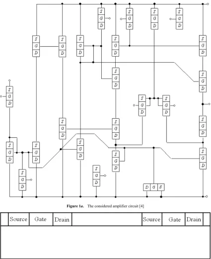
Figure 1a. The considered amplifier circuit [4]
Figure 1b. Heterostructure with two layers and sections in the epitaxial layer
2. Method
of
Solution
In this section we determine spatio-temporal distributions of concentrations of infused and implanted dopants. To determine these distributions we calculate appropriate solutions of the second Fick's law [1, 3, 18]
Boundary and initial conditions for the equations are
. (1)
(
)
=
t
t,
z
,
y
,
x
C
∂
∂
(
)
(
)
(
)
+
+
z
t,
z
,
y
,
x
C
D
z
y
t,
z
,
y
,
x
C
D
y
x
t,
z
,
y
,
x
C
D
x
C C C∂
∂
∂
∂
∂
∂
∂
∂
∂
∂
∂
, , , ,
, , C(x,y,z,0)=f (x,y,z) (2)
The function C(x,y,z,t) describes the spatio-temporal distribution of concentration of dopant; T is the temperature of annealing; DС is the dopant diffusion coefficient. Value of dopant diffusion coefficient could be changed with changing materials of heterostructure, with changing temperature of materials (including annealing), with changing concentrations of dopant and radiation defects. We approximate dependences of dopant diffusion coefficient on parameters by the following relation with account results in Refs. [20-22]
(3)
Here the function DL(x,y,z,T) describes the spatial (in heterostructure) and temperature (due to Arrhenius law) dependences of diffusion coefficient of dopant. The function P(x,y,z,T) describes the limit of solubility of dopant. Parameter γ∈[1, 3] describes average quantity of charged defects interacted with atom of dopant [20]. The function V
(x,y,z,t) describes the spatio-temporal distribution of concentration of radiation vacancies. Parameter V* describes the
equilibrium distribution of concentration of vacancies. The considered concentrational dependence of dopant diffusion coefficient has been described in details in [20]. It should be noted, that using diffusion type of doping did not generation radiation defects. In this situation ζ1= ζ2= 0. We determine spatio-temporal distributions of concentrations of radiation
defects by solving the following system of equations [21,22]
(4)
.
Boundary and initial conditions for these equations are
, , , ,
, , ρ(x,y,z,0)=fρ(x,y,z) (5)
(
)
0
0
=
∂
∂
= x
x
t,
z
,
y
,
x
C
(
)
=
0
∂
∂
=Lx
x
x
t,
z
,
y
,
x
C
(
)
0
0
=
∂
∂
= y
y
t,
z
,
y
,
x
C
(
)
=
0
∂
∂
=Ly x
y
t,
z
,
y
,
x
C
(
)
0
0
=
∂
∂
= z
z
t,
z
,
y
,
x
C
(
)
=
0
∂
∂
=Lz x
z
t,
z
,
y
,
x
C
(
)
(
(
)
)
(
)
(
( )
)
+
+
+
=
L1
1
1 * 2 2 * 2C
V
t,
z
,
y
,
x
V
V
t,
z
,
y
,
x
V
T
,
z
,
y
,
x
P
t,
z
,
y
,
x
C
T
,
z
,
y
,
x
D
D
ξ
γγς
ς
(
)
(
) (
)
(
) (
)
+
∂
∂
∂
∂
+
∂
∂
∂
∂
=
∂
∂
y
t,
z
,
y
,
x
I
T
,
z
,
y
,
x
D
y
x
t,
z
,
y
,
x
I
T
,
z
,
y
,
x
D
x
t
t,
z
,
y
,
x
I
I I
(
) (
)
−
(
) (
) (
)
−
∂
∂
∂
∂
+
k
x
,
y
,
z
,
T
I
x
,
y
,
z
t,
V
x
,
y
,
z
t,
z
t,
z
,
y
,
x
I
T
,
z
,
y
,
x
D
z
I I,V(
x
,
y
,
z
,
T
) (
I
x
,
y
,
z
t,
)
k
II, 2−
(
)
(
) (
)
(
) (
)
+
∂
∂
∂
∂
+
∂
∂
∂
∂
=
∂
∂
y
t,
z
,
y
,
x
V
T
,
z
,
y
,
x
D
y
x
t,
z
,
y
,
x
V
T
,
z
,
y
,
x
D
x
t
t,
z
,
y
,
x
V
V V
(
) (
)
−
(
) (
) (
)
+
∂
∂
∂
∂
+
k
x
,
y
,
z
,
T
I
x
,
y
,
z
t,
V
x
,
y
,
z
t,
z
t,
z
,
y
,
x
V
T
,
z
,
y
,
x
D
z
V I,V(
x
,
y
,
z
,
T
) (
V
x
,
y
,
z
t,
)
k
V,V 2+
(
)
0
0
=
∂
∂
= x
x
t,
z
,
y
,
x
ρ
(
)
=
0
∂
∂
=Lx x
x
t,
z
,
y
,
x
ρ
(
)
0
0
=
∂
∂
= y
y
t,
z
,
y
,
x
ρ
(
)
=
0
∂
∂
=Ly y
y
t,
z
,
y
,
x
ρ
(
)
0
0
=
∂
∂
= z
z
t,
z
,
y
,
x
ρ
(
)
=
0
∂
∂
=Lz z
z
t,
z
,
y
,
x
Here ρ=I,V. The function I (x,y,z,t) describes the spatio-temporal distribution of concentration of radiation interstitials;
Dρ(x,y,z,T) are the diffusion coefficients of point radiation defects; terms V2(x,y,z,t) and I2(x,y,z,t) correspond to generation divacancies and diinterstitials; kI,V(x,y,z,T) is the parameter of recombination of point radiation defects;
kI,I(x,y,z,T) and kV,V(x,y,z,T) are the parameters of generation of simplest complexes of point radiation defects.
Further we determine distributions in space and time of concentrations of divacancies ΦV(x,y,z,t) and diinterstitials ΦI(x,y,z,t) by solving the following system of equations [21,22]
(6)
.
Boundary and initial conditions for these equations are
, , , ,
, ,
ΦI(x,y,z,0)=fΦI(x,y,z), ΦV(x,y,z,0)=fΦV(x,y,z). (7)
Here DΦρ(x,y,z,T)arethediffusioncoefficientsoftheabovecomplexes of radiation defects; kI(x,y,z,T) and kV (x,y,z,T) are the parameters of decay of these complexes.
We calculate distributions of concentrations of point radiation defects in space and time by recently elaborated approach [18]. The approach based on transformation of approximations of diffusion coefficients in the following form:
Dρ(x,y,z,T)=D0ρ[1+ερgρ(x,y,z,T)], where D0ρ are the average values of diffusion coefficients, 0≤ερ<1, |gρ(x, y,z,T)|≤1, ρ =I,V. We also used analogous transformation of approximations of parameters of recombination of point defects and parameters of generation of their complexes: kI,V(x,y,z,T)=k0I,V[1+εI,V gI,V(x,y,z,T)], kI,I(x,y,z,T)=k0I,I [1+εI,I gI,I(x,y,z,T)] and
kV,V(x,y,z,T)=k0V,V [1+εV,V gV,V(x,y,z,T)], where k0ρ1,ρ2 are the their average values, 0≤εI,V <1, 0≤εI,I <1, 0≤εV,V<1, |
gI,V(x,y,z,T)|≤1, | gI,I(x,y,z,T)|≤1, |gV,V(x,y,z,T)|≤1. Let us introduce the following dimensionless variables:
, , ,
, , χ=x/Lx, η=y /Ly, φ=z/Lz. The introduction leads to transformation of Eqs.(4) and conditions (5) to the following form
(
)
(
)
(
)
(
)
(
)
+
Φ
+
Φ
=
Φ
Φ
Φ
y
t,
z
,
y
,
x
T
,
z
,
y
,
x
D
y
x
t,
z
,
y
,
x
T
,
z
,
y
,
x
D
x
t
t,
z
,
y
,
x
II I
I I
∂
∂
∂
∂
∂
∂
∂
∂
∂
∂
(
)
(
)
k
(
x
,
y
,
z
,
T
) (
I
x
,
y
,
z
t,
)
k
(
x
,
y
,
z
,
T
) (
I
x
,
y
,
z
t,
)
z
t,
z
,
y
,
x
T
,
z
,
y
,
x
D
z
I I
+
II,−
I
Φ
+
Φ 2∂
∂
∂
∂
(
)
(
)
(
)
(
)
(
)
+
Φ
+
Φ
=
Φ
Φ
Φ
y
t,
z
,
y
,
x
T
,
z
,
y
,
x
D
y
x
t,
z
,
y
,
x
T
,
z
,
y
,
x
D
x
t
t,
z
,
y
,
x
VV V
V V
∂
∂
∂
∂
∂
∂
∂
∂
∂
∂
(
)
(
)
k
(
x
,
y
,
z
,
T
) (
V
x
,
y
,
z
t,
)
k
(
x
,
y
,
z
,
T
) (
V
x
,
y
,
z
t,
)
z
t,
z
,
y
,
x
T
,
z
,
y
,
x
D
z
V V
+
V,V−
V
Φ
+
Φ2
∂
∂
∂
∂
(
)
0
0
=
∂
Φ
∂
= x
x
t,
z
,
y
,
x
ρ
(
)
=
0
∂
Φ
∂
=Lx x
x
t,
z
,
y
,
x
ρ
(
)
0
0
=
∂
Φ
∂
= y
y
t,
z
,
y
,
x
ρ
(
)
=
0
∂
Φ
∂
=Ly y
y
t,
z,
y
,x
ρ(
)
0
0
=
∂
Φ
∂
= z
z
t,
z
,
y
,
x
ρ
(
)
=
0
∂
Φ
∂
=Lz z
z
t,
z,
y
,
x
ρ
(
x
,
y
,
z
t,
) (
I
x
,
y
,
z
t,
)
I
*I~
=
V~
(
x
,
y
,
z
t,
)
=
=
V
(
x
,
y
z,
t,
)
V
*V I V
,
I
D
D
k
L
0 0 0 2=
ω
V I ,
D
D
k
L
0 0 02 ρ ρ ρ
=
Ω
20
0
D
t
L
D
I V=
ϑ
(
)
[
(
)
]
(
)
{
[
+
(
)
]
×
∂
∂
+
∂
∂
+
∂
∂
=
∂
∂
g
,
,
,
T
I~
,
,
,
g
,
,
,
T
D
D
D
,
,
,
I~
I I I
I V
I
I
ε
χ
η
φ
η
χ
ϑ
φ
η
χ
φ
η
χ
ε
χ
ϑ
ϑ
φ
η
χ
1
1
0 0
0
(
)
[
(
)
]
(
)
−
(
)
×
∂
∂
+
∂
∂
+
∂
∂
×
χ
η
φ
ϑ
φ
ϑ
φ
η
χ
φ
η
χ
ε
φ
η
ϑ
φ
η
χ
g
,
,
,
T
I~
,
,
,
I~
,
,
,
D
D
D
D
D
D
,
,
,
I~
I I V
I I
V I
I
1
0 0
0 0
(8)
, , , ,
, , (9)
We determine solutions of Eqs.(8) with conditions (9) framework recently introduced approach [18], i.e. as the power series
(10) Substitution of the series (10) into Eqs.(8) and conditions (9) gives us possibility to obtain equations for initial-order approximations of concentration of point defects and and corrections for them
and , i≥1, j≥1, k≥1. The equations are presented in the Appendix. Solutions of the equations could be obtained by standard Fourier approach [24,25]. The solutions are presented in the Appendix.
Now we calculate distributions of concentrations of simplest complexes of point radiation defects in space and time. To determine the distributions we transform approximations of diffusion coefficients in the following form:
DΦρ(x,y,z,T)=D0Φρ[1+ εΦρgΦρ(x,y,z,T)], where D0Φρ are the average values of diffusion coefficients. In this situation the Eqs.(6) could be written as
.
Farther we determine solutions of above equations as the following power series
(
)
[
ε
χ
η
φ
]
(
χ
η
φ
ϑ
)
[
ε
(
χ
η
φ
)
]
(
χ
η
φ
ϑ
)
ω
1
+
I,Vg
I,V,
,
,
T
V~
,
,
,
−
Ω
I1
+
II,g
II,,
,
,
T
I~
2,
,
,
×
(
)
[
(
)
]
(
)
{
[
+
(
)
]
×
∂
∂
+
∂
∂
+
∂
∂
=
∂
∂
g
,
,
,
T
V~
,
,
,
g
,
,
,
T
D
D
D
,
,
,
V~
V V V
V V
I
V
ε
χ
η
φ
η
χ
ϑ
φ
η
χ
φ
η
χ
ε
χ
ϑ
ϑ
φ
η
χ
1
1
0 0
0
(
)
[
(
)
]
(
)
−
(
)
×
∂
∂
+
∂
∂
+
∂
∂
×
χ
η
φ
ϑ
φ
ϑ
φ
η
χ
φ
η
χ
ε
φ
η
ϑ
φ
η
χ
g
,
,
,
T
V~
,
,
,
I~
,
,
,
D
D
D
D
D
D
,
,
,
V~
V V V
I V
V I
V
1
0 0
0 0
0 0
(
)
[
ε
χ
η
φ
]
(
χ
η
φ
ϑ
)
[
ε
(
χ
η
φ
)
]
(
χ
η
φ
ϑ
)
ω
I,Vg
I,V,
,
,
T
V~
,
,
,
V V,Vg
V,V,
,
,
T
V~
,
,
,
21
1
+
−
Ω
+
×
(
)
0
0
=
∂
∂
= χ
χ
ϑ
φ
η
χ
ρ
~
,
,
,
(
)
0
1
=
∂
∂
= χ
χ
ϑ
φ
η
χ
ρ
~
,
,
,
(
)
0
0
=
∂
∂
= η
η
ϑ
φ
η
χ
ρ
~
,
,
,
(
)
0
1
=
∂
∂
= η
η
ϑ
φ
η
χ
ρ
~
,
,
,
(
)
0
0
=
∂
∂
= φ
φ
ϑ
φ
η
χ
ρ
~
,
,
,
(
)
0
1
=
∂
∂
= φ
φ
ϑ
φ
η
χ
ρ
~
,
,
,
(
)
(
)
*
,
,
,
f
,
,
,
~
ρ
ϑ
φ
η
χ
ϑ
φ
η
χ
ρ
=
ρ(
)
=
∑ ∑
∞∑Ω
(
)
= ∞
= ∞
=
0 0 0
i j k ijk
k j
i
~
,
,
,
,
,
,
~
χ
η
φ
ϑ
ε
ω
ρ
χ
η
φ
ϑ
ρ
ρ ρ(
χ
,
η
,
φ
,
ϑ
)
I~
000V~
000(
χ
,
η
,
φ
,
ϑ
)
(
χ
,
η
,
φ
,
ϑ
)
I~
ijkV~
ijk(
χ
,
η
,
φ
,
ϑ
)
(
)
[
(
)
]
(
)
+
(
) (
)
+
+
Φ
=
Φ
Φ Φ
Φ
k
x
,
y
,
z
,
T
I
x
,
y
,
z
t,
x
t,
z
,
y
,
x
T
,
z
,
y
,
x
g
x
D
t
t,
z
,
y
,
x
I, I I
I I I
I 2
0
1
∂
∂
ε
∂
∂
∂
∂
(
)
[
]
(
)
[
(
)
]
(
)
−
+
Φ
+
+
Φ
+
Φ Φ Φ Φ Φ Φz
t,
z,
y
,
x
T
,z
,
y
,
x
g
z
D
y
t,
z,
y
,
x
T
,z
,
y
,
x
g
y
D
II I I
I I
I
I
∂
∂
ε
∂
∂
∂
∂
ε
∂
∂
1
1
0 0
(
x
,
y
,
z
,
T
) (
I
x
,
y
,
z
t,
)
k
I−
(
)
[
(
)
]
(
)
+
(
) (
)
+
+
Φ
=
Φ
Φ Φ
Φ
k
x
,
y
,
z
,
T
I
x
,
y
,
z
t,
x
t,
z
,
y
,
x
T
,
z
,
y
,
x
g
x
D
t
t,
z
,
y
,
x
I, I V
V V V
V 2
0
1
∂
∂
ε
∂
∂
∂
∂
(
)
[
]
(
)
[
(
)
]
(
)
−
+
Φ
+
+
Φ
+
Φ Φ Φ Φ Φ Φz
t,
z,
y
,
x
T
,z
,
y
,
x
g
z
D
y
t,
z,
y
,
x
T
,z
,
y
,
x
g
y
D
VV V V
V V
V
V
∂
∂
ε
∂
∂
∂
∂
ε
∂
∂
1
1
0 0
(
x
,
y
,
z
,
T
) (
I
x
,
y
,
z
t,
)
k
I(11) Now we used the series (11) into Eqs.(6) and appropriate boundary and initial conditions. The using gives the possibility to obtain equations for initial-order approximations of concentrations of complexes of defects Φρ0(x,y,z,t), corrections for them Φρi(x,y,z,t) (for them i≥1) and boundary and initial conditions for them. We remove equations and conditions to the Appendix. Solutions of the equations have been calculated by standard approaches [24,25] and presented in the Appendix.
Now we calculate distribution of concentration of dopant in space and time by using the approach, which was used for analysis of radiation defects. To use the approach we consider following transformation of approximation of dopant diffusion coefficient: DL(x,y,z,T)=D0L[1+
εLgL(x,y,z,T)], where D0L is the average value of dopant diffusion coefficient, 0≤εL<1, |gL(x,y,z,T)|≤1. Farther we consider solution of Eq.(1) as the following series:
Using the relation into Eq.(1) and conditions (2) leads to obtaining equations for the functions Cij(x,y,z,t) (i ≥1, j ≥1), boundary and initial conditions for them. The equations are presented in the Appendix. Solutions of the equations have been calculated by standard approaches (see, for example, [24,25]). The solutions are presented in the Appendix.
We analyzed distributions of concentrations of dopant and radiation defects in space and time analytically by using the second-order approximations on all parameters,
which have been used in appropriate series. Usually the second-order approximations are enough good approximations to make qualitative analysis and to obtain quantitative results. All analytical results have been checked by numerical simulation.
3. Discussion
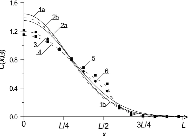
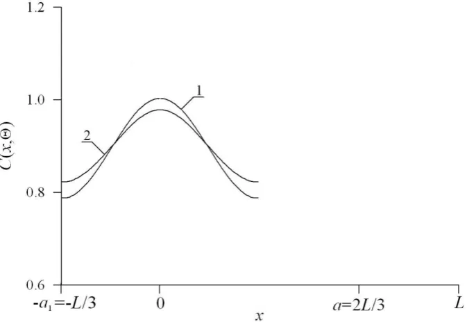
In this section we analyzed spatio-temporal distributions of concentrations of dopants. Figs. 2 shows typical spatial distributions of concentrations of dopants in neighborhood of interfaces of heterostructures. We calculate these distributions of concentrations of dopants under the following condition: value of dopant diffusion coefficient in doped area is larger, than value of dopant diffusion coefficient in nearest areas. In this situation one can find increasing of compactness of field-effect transistors with increasing of homogeneity of distribution of concentration of dopant at one time. Changing relation between values of dopant diffusion coefficients leads to opposite result (see Figs 3).
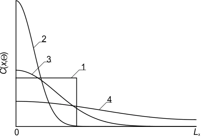
It should be noted, that framework the considered approach one shall optimize annealing of dopant and/or radiation defects. To do the optimization we used recently introduced criterion [26-34]. The optimization based on approximation real distribution by step-wise function ψ (x,y,z) (see Figs. 4). Farther the required values of optimal annealing time have been calculated by minimization the following mean-squared error
[image:6.595.149.457.478.698.2](12)
Figure 2a. Dependences of concentration of dopant, infused in heterostructure from Figs. 1, on coordinate in direction, which is perpendicular to interface between epitaxial layer substrate. Difference between values of dopant diffusion coefficient in layers of heterostructure increases with increasing of number of curves. Value of dopant diffusion coefficient in the epitaxial layer is larger, than value of dopant diffusion coefficient in the substrate. Solid lines are analytical results. Dashed lines are numerical results. Squares and triangles are experimental results in homogeneous structures from [34,35], respectively
(
)
=
∑
Φ
(
)
Φ
∞=0 Φ
i i
i
x
,
y
,
z
t,
t,
z
,
y
,
x
ρ ρρ
ε
(
)
=
∑ ∑
∞(
)
= ∞
=
0 1
i j ij
j i
L
C
x
,
y
,
z
t,
t,
z
,
y
,
x
C
ε
ξ
(
)
(
)
[
]
∫ ∫ ∫ Θ − = L L Lx y z
z y x
x d y d z d z , y , x ,
z , y , x C L L L U
0 0 0
1 ψ
x
0.0 0.4 0.8 1.2 1.6
C
(
x
,
Θ
)
>
L
/4
L
/2
0
3
L
/4
L
1a
1b 2b
2a
3 4
Figure 2b. Dependences of concentration of dopant, implanted in heterostructure from Figs. 1, on coordinate in direction, which is perpendicular to interface between epitaxial layer substrate. Difference between values of dopant diffusion coefficient in layers of heterostructure increases with increasing of number of curves. Value of dopant diffusion coefficient in the epitaxial layer is larger, than value of dopant diffusion coefficient in the substrate. Curve 1 corresponds to homogenous sample and annealing time Θ=0.0048(Lx2+Ly2+Lz2)/D0. Curve 2 corresponds to homogenous sample and
annealing time Θ=0.0057(Lx2+Ly2+Lz2)/D0. Curves 3 and 4 correspond to heterostructure from Figs. 1; annealing times Θ=0.0048(Lx2+Ly2+Lz2)/D0 and Θ
=0.0057(Lx2 +Ly2+Lz2)/D0, respectively. Solid lines are analytical results. Dashed lines are numerical results. Squares and triangles are experimental
results in homogeneous structures from [36,37], respectively
[image:7.595.132.469.404.636.2]Figure 3b. Calculated distributions of implanted dopant in epitaxial layers of heterostructure. Solid lines are spatial distributions of implanted dopant in system of two epitaxial layers. Dushed lines are spatial distributions of implanted dopant in one epitaxial layer. Annealing time increases with increasing of number of curves
Figure 4a. Distributions of concentration of infused dopant in depth of heterostructure from Fig. 1 for different values of annealing time (curves 2-4) and idealized step-wise approximation (curve 1). Increasing of number of curve corresponds to increasing of annealing time
x
0.00000
0.00001
0.00010
0.00100
0.01000
0.10000
1.00000
C
(
x
,
Θ
)
fC
(
x
)
L
/4
0
L
/2
x
03
L
/4
L
1
2
Substrate
Epitaxial
layer 1
Epitaxial
layer 2
C
(
x
,
Θ
)
0
L
x2
1
3
[image:8.595.131.471.368.598.2]Figure 4b. Distributions of concentration of implanted dopant in depth of heterostructure from Fig. 1 for different values of annealing time (curves 2-4) and idealized step-wise approximation (curve 1). Increasing of number of curve corresponds to increasing of annealing time
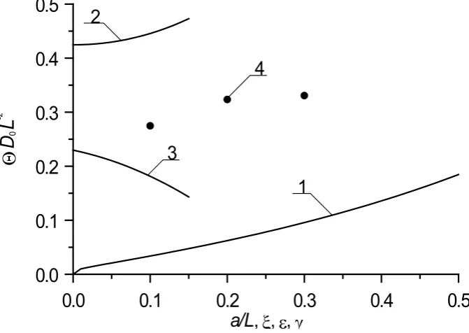
Figure 5a. Dimensionless optimal annealing time of infused dopant as a function of several parameters. Curve 1 describes the dependence of the annealing time on the relation a/L and ξ=γ=0 for equal to each other values of dopant diffusion coefficient in all parts of heterostructure. Curve 2 describes the dependence of the annealing time on value of parameter ε for a/L=1/2 and ξ=γ=0. Curve 3 describes the dependence of the annealing time on value of parameter ξ for a/L=1/2 and ε=γ=0. Curve 4 describes the dependence of the annealing time on value of parameter γ for a/L=1/2 and ε=ξ= 0
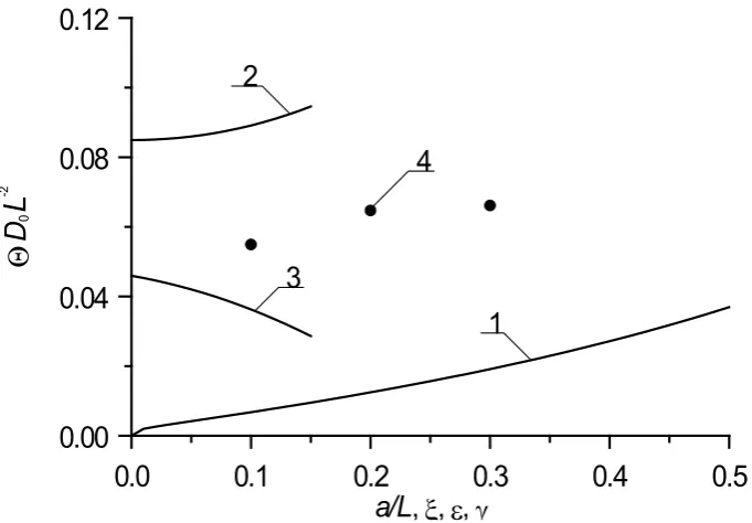
We show optimal values of annealing time as functions of parameters on Figs. 5. It is known, that standard step of manufactured ion-doped structures is annealing of radiation defects. In the ideal case after finishing the annealing dopant achieves interface between layers of heterostructure. If the dopant has no enough time to achieve the interface, it is practicably to anneal the dopant additionally. The Fig. 5b shows the described dependences of optimal values of additional annealing time for the same parameters as for Fig. 5a. Necessity to anneal radiation defects leads to smaller values of optimal annealing of implanted dopant in comparison with optimal annealing time of infused dopant.
x
C
(
x
,
Θ
)
1
2
3
4
0
L
0.0
0.1
0.2
0.3
0.4
0.5
a/L
,
ξ
,
ε
,
γ
0.0
0.1
0.2
0.3
0.4
0.5
Θ
D
0L
-2
3
2
4
[image:9.595.131.467.364.602.2]Figure 5b. Dimensionless optimal annealing time of implanted dopant as a function of several parameters. Curve 1 describes the dependence of the annealing time on the relation a/L and ξ=γ=0 for equal to each other values of dopant diffusion coefficient in all parts of heterostructure. Curve 2 describes the dependence of the annealing time on value of parameter ε for a/L=1/2 and ξ=γ=0. Curve 3 describes the dependence of the annealing time on value of parameter ξ for a/L=1/2 and ε=γ=0. Curve 4 describes the dependence of the annealing time on value of parameter γ for a/L=1/2 and ε=ξ= 0
4. Conclusions
In this paper we introduce an approach to increase integration rate of element of an operational amplifier circuit. The approach gives us possibility to decrease area of the elements with smaller increasing of the element’s thickness.
Appendix
Equations for the functions and , i≥0, j≥0, k≥0 and conditions for them
;
, i≥1,
0.0
0.1
0.2
0.3
0.4
0.5
a/L
,
ξ
,
ε
,
γ
0.00
0.04
0.08
0.12
Θ
D
0L
-2
3
2
4
1
(
χ
,
η
,
φ
,
ϑ
)
I~
ijkV~
ijk(
χ
,
η
,
φ
,
ϑ
)
(
)
(
)
(
)
(
)
∂
∂
+
∂
∂
+
∂
∂
=
∂
∂
2 000 2
2 000 2
2 000 2
0 0 000
φ
ϑ
φ
η
χ
η
ϑ
φ
η
χ
χ
ϑ
φ
η
χ
ϑ
ϑ
φ
η
χ
I~
,
,
,
I~
,
,
,
I~
,
,
,
D
D
,
,
,
I~
V I
(
)
(
)
(
)
(
)
∂
∂
+
∂
∂
+
∂
∂
=
∂
∂
2 000 2
2 000 2
2 000 2
0 0 000
φ
ϑ
φ
η
χ
η
ϑ
φ
η
χ
χ
ϑ
φ
η
χ
ϑ
ϑ
φ
η
χ
V~
,
,
,
V~
,
,
,
V~
,
,
,
D
D
,
,
,
V~
I V
(
)
(
)
(
)
(
)
+
×
∂
∂
+
∂
∂
+
∂
∂
=
∂
∂
V I i
i i
V I i
D
D
,
,
,
I~
,
,
,
I~
,
,
,
I~
D
D
,
I~
0 0 2
00 2 2
00 2 2
00 2
0 0 00
φ
ϑ
φ
η
χ
η
ϑ
φ
η
χ
χ
ϑ
φ
η
χ
ϑ
ϑ
χ
(
)
(
)
(
)
(
)
+
∂
∂
∂
∂
+
∂
∂
∂
∂
×
− −η
ϑ
φ
η
χ
φ
η
χ
η
χ
ϑ
φ
η
χ
φ
η
χ
χ
,
,
,
I~
T
,
,
,
g
,
,
,
I~
T
,
,
,
g
iI i
I 100 100
(
)
(
)
∂
∂
∂
∂
+
−φ
ϑ
φ
η
χ
φ
η
χ
φ
,
,
,
I~
T
,
,
,
g
i,i≥1, ; ; ;
(
)
(
)
(
)
(
)
(
)
× ∂ ∂ + ∂ ∂ + ∂ ∂ + ∂ ∂ = ∂ ∂ T g V V V D D V V i i i I Vi , ~ , , , ~ , , , ~ , , , , , ,
~ 2 00 2 2 00 2 2 00 2 0 0
00 χ η φ
χ φ ϑ φ η χ η ϑ φ η χ χ ϑ φ η χ ϑ ϑ χ
(
)
(
)
(
)
(
)
× ∂ ∂ + ∂ ∂ ∂ ∂ + ∂ ∂× − g T V− g T
D D D D V V i V I V I V
i , , , , , , ~ , , , , , ,
~ 100 0 0 0 0
100 χ η φ
φ η ϑ φ η χ φ η χ η χ ϑ φ η χ
(
)
I V i D D V 0 0 100 , , ,~ ∂ ∂ × − φ ϑ φ η χ
(
)
(
)
(
)
(
)
− ∂ ∂ + ∂ ∂ + ∂ ∂ = ∂ ∂ 2 010 2 2 010 2 2 010 2 0 0010 , , , ~ , , , ~ , , , ~ , , ,
~
φ
ϑ
φ
η
χ
η
ϑ
φ
η
χ
χ
ϑ
φ
η
χ
ϑ
ϑ
φ
η
χ
I I ID D I V I
(
)
[
1
+
ε
I,Vg
I,Vχ
,
η
,
φ
,
T
]
I
~
000(
χ
,
η
,
φ
,
ϑ
)
V
~
000(
χ
,
η
,
φ
,
ϑ
)
−
(
)
(
)
(
)
(
)
−
∂
∂
+
∂
∂
+
∂
∂
=
∂
∂
2 010 2 2 010 2 2 010 2 0 0 010φ
ϑ
φ
η
χ
η
ϑ
φ
η
χ
χ
ϑ
φ
η
χ
ϑ
ϑ
φ
η
χ
V~
,
,
,
V~
,
,
,
V~
,
,
,
D
D
,
,
,
V~
I V(
)
[
1
+
ε
I,Vg
I,Vχ
,
η
,
φ
,
T
]
I~
000(
χ
,
η
,
φ
,
ϑ
) (
V~
000χ
,
η
,
φ
,
ϑ
)
−
(
)
(
)
(
)
(
)
−
∂
∂
+
∂
∂
+
∂
∂
=
∂
∂
2 020 2 2 020 2 2 020 2 0 0 020φ
ϑ
φ
η
χ
η
ϑ
φ
η
χ
χ
ϑ
φ
η
χ
ϑ
ϑ
φ
η
χ
I~
,
,
,
I~
,
,
,
I~
,
,
,
D
D
,
,
,
I~
V I(
)
[
1
+
ε
I,Vg
I,Vχ
,
η
,
φ
,
T
]
[
I~
010(
χ
,
η
,
φ
,
ϑ
) (
V~
000χ
,
η
,
φ
,
ϑ
)
+
I~
000(
χ
,
η
,
φ
,
ϑ
) (
V~
010χ
,
η
,
φ
,
ϑ
)
]
−
(
)
(
)
(
)
(
)
−
∂
∂
+
∂
∂
+
∂
∂
=
∂
∂
2 020 2 2 020 2 2 020 2 0 0 020φ
ϑ
φ
η
χ
η
ϑ
φ
η
χ
χ
ϑ
φ
η
χ
ϑ
ϑ
φ
η
χ
V~
,
,
,
V~
,
,
,
V~
,
,
,
D
D
,
,
,
V~
V I(
)
[
1+ε
I,VgI,Vχ
,η
,φ
,T]
[
I~010(
χ
,η
,φ
,ϑ
) (
V~000χ
,η
,φ
,ϑ
)
+~I000(
χ
,η
,φ
,ϑ
) (
V~010χ
,η
,φ
,ϑ
)
]
−
(
)
(
)
(
)
(
)
− ∂ ∂ + ∂ ∂ + ∂ ∂ = ∂ ∂ 2 001 2 2 001 2 2 001 2 0 0001 , , , ~ , , , ~ , , , ~ , , ,
~
φ
ϑ
φ
η
χ
η
ϑ
φ
η
χ
χ
ϑ
φ
η
χ
ϑ
ϑ
φ
η
χ
I I ID D I V I
(
)
[
1ε
χ
,η
,φ
,]
~2(
χ
,η
,φ
,ϑ
)
000,
,IgII T I I + −
(
)
(
)
(
)
(
)
− ∂ ∂ + ∂ ∂ + ∂ ∂ = ∂ ∂ 2 001 2 2 001 2 2 001 2 0 0001 , , , ~ , , , ~ , , , ~ , , ,
~
φ
ϑ
φ
η
χ
η
ϑ
φ
η
χ
χ
ϑ
φ
η
χ
ϑ
ϑ
φ
η
χ
V V VD D V I V
(
)
[
1
+
ε
I I,g
II,χ
,
η
,
φ
,
T
]
V~
0002(
χ
,
η
,
φ
,
ϑ
)
−
(
)
(
)
(
)
(
)
+
×
∂
∂
+
∂
∂
+
∂
∂
=
∂
∂
V I V ID
D
,
,
,
I~
,
,
,
I~
,
,
,
I~
D
D
,
,
,
I~
0 0 2 110 2 2 110 2 2 110 2 0 0 110φ
ϑ
φ
η
χ
η
ϑ
φ
η
χ
χ
ϑ
φ
η
χ
ϑ
ϑ
φ
η
χ
(
)
(
)
(
)
(
)
[
(
)
× ∂ ∂ + ∂ ∂ ∂ ∂ + ∂ ∂ ∂ ∂× gI T I gI T I gI , , ,T
, , , ~ , , , , , , ~ , ,
, 010 010