Optimal Controller of a PV Grid Connected Two Area Power System

(1)

Optimal Controller of a PV Grid Connected Two-Area Power System

Samar Emara

1

_{, Abdulla Ismail}

2

_{, Ali Sayyad}

3

1_{Graduate Student, Department of Electrical Engineering and Computing Sciences, RIT, Dubai, UAE} 2_{Professor, Department of Electrical Engineering and Computing Sciences, RIT, Dubai, UAE}

3_{Lecturer, Department of Electrical Engineering and Computing Sciences, RIT, Dubai, UAE}

***Abstract

-In this paper, a PV grid connected two-area power system with 45% penetration level is presented. The model of the two-area system is explained in detail and the system frequency errors due to load changes are studied. The design of an optimal linear quadratic regulator (LQR) is presented as the tool to regulate those errors, and so to keep the system response within the required specifications: settling time less than 3s, undershoot less than 0.02 Hz and steady state error equal to zero. The design of a conventional PI controller is also explained for the same system. Finally, the system responses due to LQR and PI controllers are compared.

Key Words: optimal, control, LQR, PI, power system, PV system.

1.INTRODUCTION

As the contribution of renewable energy is becoming an essential part of the power generation, it is of critical importance to study the effects of this increased penetration of the renewable energy resources on the power system and study the potential problems associated with it. The load frequency control (LFC) is one of the main elements to be considered in the study of this interconnected system. [1] In this paper, a well-structured LQR controller has been designed to assure a continuous and steady system performance through system frequency control.

Section 2 of this paper represents the model of the two-area power system connected to PV system. Section 3 explains the LQR and PI controllers design details and their relative system responses. The comparison between the response of the uncontrolled system and the controlled system is presented in section 4. In addition, this section will include the comparison between the responses for the system with the conventional PI controller and that with LQR included.

2.MODEL OF THE TWO-AREA POWER SYSTEM

The main components of a thermal power plant are: The governor which is used to monitor and measure the system speed changes and to control the valve. The turbine transforms the input energy (in this case coming from the

steam) into mechanical energy that goes into the generator to produce electrical energy. The reheater makes the system more efficient as it reheats the steam to keep the same high temperature of the steam that entered the governor. [2]

In this section the specific mathematical model of each area has been presented along with the connection of these two areas in one system and the response of this system without controllers. The final model is shown with the photovoltaic system connected to it. The PV system has been designed separately based on [ 3] but is not the focus of this paper. The integral controller is required in both areas to eliminate the steady state error. Since the integral controller adds one state variable to the model of the system, it has been included to the models of both areas for which the LQR controller is designed.

2.1Mathematical Model of Area 1

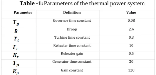
[image:1.595.301.567.460.588.2]

The state model of the first area in this thermal power system with integral controller is presented here. Table 1 shows the parameters that were used in this modeling.

Table -1:Parameters of the thermal power system

Parameter Definition Value

Governor time constant 0.08

Droop 2.4

Turbine time constant 0.3

Reheater time constant 10

Reheater gain 0.5

Generator time constant 20

Gain constant 120

(2)

Accordingly, the state model of the thermal power system with an integral controller becomes the following.

2.2 Model of the Second Area

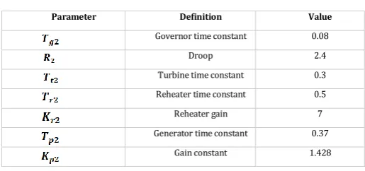
Table -2: Parameters of area 2 model.

Parameter Definition Value

Governor time constant 0.08

Droop 2.4

Turbine time constant 0.3 Reheater time constant 0.5

Reheater gain 7

Generator time constant 0.37

[image:2.595.37.579.45.208.2]

Gain constant 1.428

Table 2 shows the parameter from which the state model of area 2 has been constructed and Figure 2 shows the block diagram. The state space equations of this power system have been calculated as follows (Equations 8-12).

(1)

[image:2.595.306.564.279.400.2]

(2)

Fig -1: Block diagram of area 1.

(3)

(4)

(5)

(6)

(7)

Fig -2: Block diagram of area 2 in the thermal power system.

(8) (9)

[image:2.595.34.569.452.757.2]

(3)

In matrix form, we have

2.3 Two-Area System

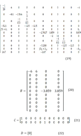
For the connected two-area system, there are 5 state variables relative to the first area and other 5 state variables related to the second one. However, the transmission line connecting the two areas adds one more state variable to represent the tie-line power change giving a total of 11 state variables. For each area, one input is the change of load power and another input is from the PV system connected to the grid. Therefore, for this interconnected system, it has 4

inputs ( , , & ) and 2 outputs

which are the change in frequency of area 1 ( )

represented by the 1st_{state variable and the change in}

frequency of area 2 ( ) represented by the 6th_state

variable.

The full mathematical calculations are presented as follows. Note that equations 15 to 18 are the modified equations for the full model of the two-area system to account for the interconnection between both areas. The state model of the two-area system connected to PV is shown in matrices 19-22.

The system state matrix (A)=

[image:3.595.313.581.118.565.2]

The controllability and observability of the system have also been checked and the two-area system is controllable and observable. As to the stability of the two-area system, the closed loop poles were also checked, and the system is stable. Figure 3 shows the frequency error of the two-area system without any controller (without even the integral controller), Figure 4 and Figure 5 show the frequency error response of both outputs in this system with integral controller for various changes in load (reasonable change in load and an extreme change in load (50%)). Figure 6 shows the block diagram of the interconnected two-area system with PV with integral controllers only.

(11)

(12)

(13)

(14)

(15)

(16)

(18)

(20)

(21)

(22)

(17)

(4)

[image:4.595.36.291.88.275.2]

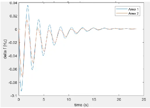
[image:4.595.37.288.319.500.2]

Fig -3: Response of the two-area system without any controller due to 50% increase in load.

Fig -4: Change of frequency of both areas (for the system with integral controller only) for 20% increase in load.

It is observed that without using the integral controller the steady state frequency error does not reach zero, which is highly undesirable. When including the integral controller, the steady state error requirement is met, however the settling time is much larger than the required 3s (it is more than 18s in both cases) and the undershoot is also much larger than the required 0.02 Hz. The second case of a sudden increase in load, equal to 50%, is an extreme case. However, even in the first case (i.e. reasonable change in load power), neither the undershoot nor the settling time criteria were met with integral controller only. Thus, LQR and PI controllers are designed to enhance the system frequency performance.

standard optimal controller technique. To design the optimal controller, a performance measure or cost function should be chosen, which is the parameter that is required to be minimized by the optimal controller. [4]

A certain state trajectory is defined after applying the controller signal obtained from the optimal controller over a certain period of time along with an initial state for the system at (to). [4] The optimal control problem is defined as finding a control (u*_{) for the system in Equation 23.}

which makes it follow a trajectory that minimizes the targeted performance measure given in Equation 24:

z(t) represents the desired output vector and y(t) represents the output vector. Q and R are the matrices that should be chosen in order to give the minimum value of the performance index (J). Q is the error weighted matrix, and it should be positive semidefinite. The more focus is required on minimizing a certain parameter, the larger the weight that should be attributed to its corresponding state variable in the Q matrix. R is the control weighted matrix and it should be positive definite. [4]

Fig-5: Change of frequency of both areas (for the system with integral controller only) for 50% increase in load.

(23)

(24)

3.CONTROLLERS DESIGN

3.1 LQR Controller Design

[image:4.595.35.294.544.730.2]

(5)

When the optimal values of Q and R matrices are substituted in the Riccati equation (Equation 25), it solves for the optimal costate (P) matrix. [5]

This costate (P) matrix is substituted into the optimal controller equation (Equation 26) in order to determine the optimal controller ( in the form of state feedback gains (K). [5]

This negative feedback controller is used to obtain the optimal response of the system.

[image:5.595.47.559.57.612.2]

An optimal controller does not always exist for every system. In order to check if an optimal controller exists for the system under study, the controllability and observability matrices have to be obtained. If the system is completely controllable and observable, then an optimal controller can be designed Fig -6: Block Diagram of the two-area system connected with the PV system.

(25)

(6)

for this system, and the system is controllable and observable. [4]

If the system is controllable and observable, the main challenge remaining in LQR is a suitable choice of the Q and R matrices that are chosen based on the user experience. [5] An algebraic approach to calculate Q and R systematically has been provided in [7]. The idea behind this approach is to compare between the actual and the desired characteristic equations of the system.

The desired characteristic equation can be obtained for second and third order systems easily because it is pre-defined according to the specifications of undershoot and settling time required. Then, the comparison with the actual characteristic equation (in terms of P matrix elements) is possible, and the P matrix would be obtained. This would solve the Riccati equation. Based on that, and with assuming a certain value for the R matrix, the Q matrix can be obtained by calculation rather than assumption.

However, the method presented in [7] is for second and third order systems, while the system under study has an order of 11. The desired characteristic equation for higher order systems has no pre-defined equation related to the specifications (settling time and undershoot). They rather depend on the choice of the desired closed loop poles, which by their turn depend on user experience. Moreover, not all the elements in the P matrix can be obtained by the comparison of both equations leaving behind many variables that need to be tuned based on trial and error for higher order systems, which leads to a very high cost function most of the time. Therefore, the best way to design LQR based controller for a higher order system is by creating an optimization code and further tuning of the system manually according to optimization results, which has been implemented in this paper.

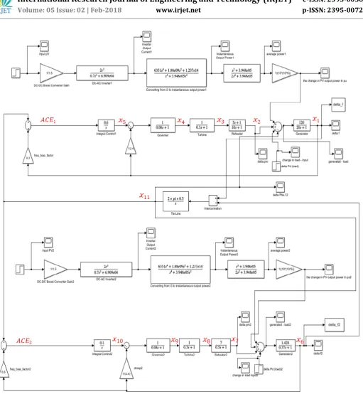
[image:6.595.305.583.354.578.2]

Figure 7 shows the response of both areas due to a reasonable change in load that is equal between both systems and Table 3 summarizes the specifications. For this case, the response is within the required performance criteria for the undershoot and the steady state error. The settling time is more than the required range due to the challenge of reaching the optimized values of Q and R with systems of complex mathematical models. However, the undershoot is minimal (already very close to 0). Thus, this increase in settling time is a tradeoff that can be accepted.

[image:6.595.34.568.637.790.2]

Fig. -7: Response of both areas with LQR controller for equal and reasonable change in load.

Table -3: Response summary for both areas with LQR (equal and reasonable change in load).

Area 1 Area 2

Settling Time (s) 8.74751 10.442

Undershoot (Hz) -0.00074147 -0.00045986

SSE (Hz) 0 0

(27)

(28)

(29)

(7)

[image:7.595.23.291.199.420.2]

[image:7.595.302.564.251.433.2]

Figure 8 shows the response of the two-area system with a sudden 50% increase in load and Table 4 shows a summary of the response. It can be noted that even under this extreme case, the undershoot and the steady state error requirements are met by the LQR controller designed. It is noticed that the settling time in all cases did not change with the changes in the load. A key improvement of the system response can be observed from the uncontrolled case.

[image:7.595.306.564.495.675.2]

Fig. -8: Response of both areas with LQR controllers for 50% change in load.

Table -4: Response summary of both areas with LQR controller for equal change in load of 50%.

Area 1 Area 2

Settling Time (s) 8.7475 10.442

Undershoot (Hz) -0.0018537 -0.0011496

SSE (Hz) 0 0

3.2 PI Controller Design

A conventional PI controller has been designed for this system in order to compare the results due to PI and LQR controllers.

By optimizing the system to get the best values of and ,

the value of , and were the result the

optimization for area 1. As to area 2, no values for were

obtained and only value existed. Any value added to area 2 made it worse in terms of undershoot and oscillations.

Therefore, only integral controller was added with the value of to the second area. Figure 9 shows the two-area system with PI controller.

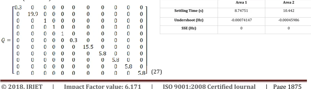
[image:7.595.36.295.505.565.2]

For the case of a reasonable increase in load that is equal in both areas, Figure 10, Figure 11 and Table 5 describe the response while Figure 12 shows the tie-line power change. This tie-line power change represents the power transferred between these two areas and it goes to 0 at steady state. [8] Area 2 satisfies the criteria of undershoot and steady state error, however, area 1 only satisfies the steady state error. Both of them have a long settling time.

Fig -10: Response of area 1 in the two-area system for a reasonable increase in load.

(8)

[image:8.595.29.572.48.615.2]

Fig -9: Block Diagram of the PV grid connected two-area power system with PI controllers.

(9)

[image:9.595.27.567.47.250.2]

Fig. -12: Tie-line power change response due to a reasonable increase in load.

Figure 13, Figure 14 and Table 6 show the response of both areas with PI controller for the extreme case of 50% increase in load. Also, the criteria required are not met. The response is slightly enhanced than the case without any controller, however, the response is still not acceptable. Figure 15 shows the tie-line power change between both areas.

Fig. -13: Response of area 1 in the two-area system for a 50% increase in load.

[image:9.595.305.575.302.442.2]

Fig. -14: Response of area 2 in the two-area system for a 50% increase in load.

Fig. -15: Tie-line power change between area 1 and area 2 for a 50% increase in load.

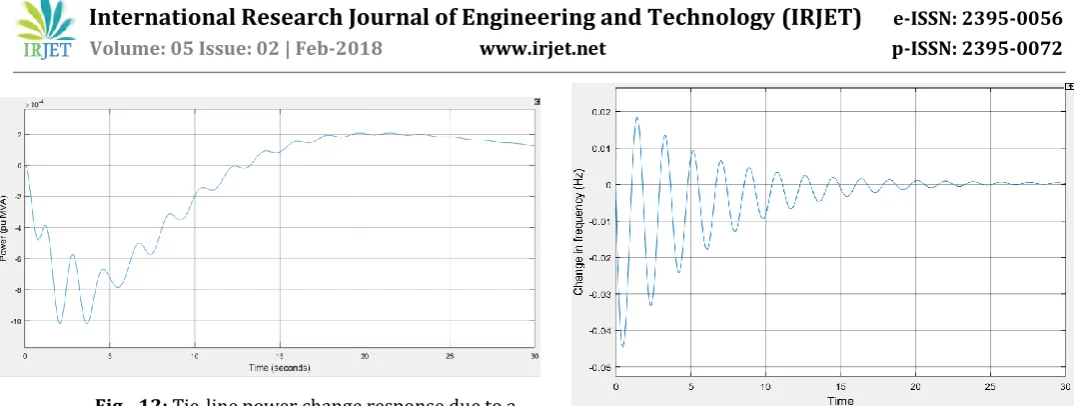
4.RESULTS AND COMPARISON ANALYSIS

Table 7 summarizes the specification values for the uncontrolled and the controlled system, along with the results due to LQR and PI controllers in order to compare between the effect of each type of controller. The response of the system frequency for both the case of the reasonable change in load and the case of an extreme change in load (50%) have also been summarized in Table 7 for comparison purposes.

Table -5: Response summary of the two-area system for a reasonable increase in load.

Area 1 Area 2

Settling Time (s) 9.59875 22.1189

Undershoot (Hz) -0.03340 -0.01788

SSE (Hz) 0 0

Table -6: Response summary for both areas due to an increase in load of 50%.

Area 1 Area 2

Settling Time (s) 9.5987 22.11898

Undershoot (Hz) -0.0835 -0.04472

[image:9.595.27.287.471.654.2]

(10)

For the LQR controlled two-area system, the system performance was enhanced considerably. The undershoot is minimal and the response is smooth with a steady state error equal to zero. Although the settling time did not meet the specification, but the undershoot is already fairly small. For example, the maximum undershoot reached was in the extreme case of 50% increase in load. This undershoot is -0.001 which means that the worst value of the frequency reached is 49.999Hz. Thus, settling time that is more than 3s to reach to zero steady state error is still acceptable. However, this also shows a limitation of LQR controller when the system becomes more complicated as the optimization becomes very difficult to implement. Thus, a response that absolutely satisfies all the criteria with LQR controller is difficult to attain.

When applying only the conventional PI controller to the system described in this paper, the system had more oscillations and worse undershoot and settling time. It did improve the system compared to the response of the uncontrolled system, however, even with the optimized values of and obtained in this work, neither the settling time nor the undershoot specifications were met. Therefore, advanced controllers such as LQR were required. It can be observed that LQR improved the oscillations and undershoot greatly compared to the system with the conventional controller (PI) only. Moreover, LQR helped satisfy two conditions absolutely and the settling time condition to a fairly acceptable extent. As to the extreme case of 50% increase in load, LQR showed a very powerful enhancement to the system performance as the undershoot of the system frequency was still kept within the required specification.

5.CONCLUSION

This paper presented a model for a two-area power system connected to PV system with 45% penetration level. An optimal controller (namely, LQR) has been designed and applied to this system in order to control the frequency of the system due to various load changes. A conventional PI controller has also been designed and the results due to both controllers have been compared. It has been observed that the conventional PI controller was not sufficient to meet the required specifications for the system frequency (undershoot less than 0.02Hz, settling time less than 3s and steady state error equal to zero) and it increased the oscillations in the system. Therefore, LQR was essential to enhance the performance; it reduced the oscillations tremendously and made the undershoot and the steady state error meet the criteria. The settling time was off the range, however, LQR was so powerful in decreasing the undershoot to a very small value (close to 0) which made this tradeoff with the settling time acceptable and does not affect the performance of the system negatively.

ACKNOWLEDGEMENT

The authors wish to thank RIT Dubai for the support.

REFERENCES

[1] A. Ikhe, A. Kulkarni, D. Veeresh, “Load frequency control

using fuzzy logic controller of two-area thermal-thermal power plant,” International Journal of Emerging Technology and Advanced Engineering, ISSN 2250-2459, vol. 2, issue 10, October 2012.

[2] A. Monti and F. Ponci, “Electric power systems”,

Intelligent Monitoring, Control, and Security of Critical

Infrastructure Systems Springer, 2015. DOI

10.1007/978-3-662-44160-2_2)

[3] M. Alam and F. Khan, “Transfer function mapping for a

grid connected PV system using reverse synthesis technique,” in 14th Workshop on Control and Modeling for Power Electronics (COMPEL)-IEEE, 2013.

[4] D. Kirk, Optimal Control Theory an Introduction,

Mineola NY: Dover Publications, 1998.

[5] B.D. Anderson and J.B. Moore, Optimal Control Linear

Quadratic Methods, New Jersey: Prentice Hall, 1989.

[6] A. Ikhe, A. Kulkarni, D. Veeresh, “Load frequency control

using fuzzy logic controller of two-area thermal-thermal power plant,” International Journal of Emerging Technology and Advanced Engineering, ISSN 2250-2459, vol. 2, issue 10, October 2012.

[7] V. Kumar, J. Jerome, K. Srikanth. “Algebraic approach for

selecting the weighting matrices of linear quadratic regulator,” in Conf. on Green Computing Communication and Electrical Engineering (ICGCCEE), Coimbatore,

India, March 2014. DOI:

[image:10.595.30.296.127.283.2]

10.1109/ICGCCEE.2014.6922382 Table -7: Comparison between the response specifications

for the uncontrolled system and due to PI and LQR

Settling Time Undershoot Steady State Error Area

1 Area 2 Area 1 Area 2 Area 1 Area 2

Case 1

(reason-able increase

in load)

PI 9.598 22.1 -0.033 -0.018 0 0

LQR 8.747 10.422 -0.0007 -0.0005 0 0

Case 2 (50% increase

in load)

Uncontrolled 23.14 20.6 -0.087 -0.067 -0.03 -0.03

I 15.11 14.1 -0.093 -0.071 0 0

PI 9.598 22.1 -0.083 -0.045 0 0

(11)

Single Area Power Generation System Using Adaptive Fuzzy Logic and PI Control,” International Research Journal of Engineering and Technology (IRJET), vol. 04, issue: 08, August 2017.

BIOGRAPHIES

Samar A. Emara Born in 1994. Graduated with BSc in Electrical Engineering from the Petroleum Institute, Abu Dhabi in 2016. Currently doing MSc in Electrical Engineering (in control systems) at RIT Dubai.

Worked as a teaching assistant for the academic year (2016-2017) at RIT Dubai and is currently a full time Master student. Samar is a student member of IEEE and has filed a patent of the project entitled (Design of Nanomagnetic Tagging and Monitoring System) in 2016.

Abdulla Ismail Professor of Electrical Engineering. Emirati citizen, Born in Sharjah. BSc (‘80), MSc (’83), and PhD (’86) in Electrical Engineering from University of Arizona, USA. 1st Emirati to hold a PhD in Engineering. Has over 30 years of teaching and research experience at UAE University (ALAIN) and RIT Dubai.

Worked as Vice Dean of College of Engineering, Advisor to the Vice Chancellor at UAE University. Worked in Education and Technology management Dubai Silicon Oasis and Emirates Foundation. Teaching and research interests in Control and Power systems, intelligent systems, smart grids, renewable energy systems modeling and control.

Coauthored two books; desalination technology in the UAE and Contemporary Scientific Issues. Published over 90 referred technical papers in local and international journals and conferences. Won Emirates Energy Award (Education and Energy Management), 2015. Won several UAEU awards for University and Community service. Won the Fulbright scholarship, USA Government. A senior member of IEEE.

A member of Dubai KHDA University Quality Assurance International Board, Chair of the Zayed Future Energy Prize (Global High Schools Committee), Chairman of AURAK Engineering Advisory Council.

Ali A. Sayyad PhD in Systems and Control Engineering, City, University of London, UK. Research interests include control system analysis and design including modelling and optimization techniques in both linear and nonlinear cases and Robust control applications

Dr. Sayyad holds more than Six years of experience in industrial field, working as an electrical and/or Control engineer. Since 2013, he has also been a member of STEM organization. Dr. Sayyad joined the Department of Electrical Engineering as an Electrical Lecturer, at Rochester Institute of Technology Dubai in September 2017.