Studying time use variations in 18 countries applying a life course perspective

Munich Personal RePEc Archive

Studying time use variations in 18

countries applying a life course

perspective

Versantvoort, Maroesjka

Department of Economics, Leiden University

2008

Online at

https://mpra.ub.uni-muenchen.de/21141/

St u dyin g t im e u se va r ia t ion s in 1 8 cou n t r ie s a pplyin g

a life cou r se pe r spe ct ive

∗

M a roe sj k a Ve r sa nt voor t

Leiden University Department of Economics

Research program Reforming Social Security P.O. Box 9520, 2300 RA Leiden, The Netherlands

Phone: ++31 71 527 4856

E-mail: [email protected]

Abst r a ct

To gain insight in variations in life courses during last decades, and the factors underlying these variations, time use data seem suited. By means of analyzing time use data insight is gained in the (relative) importance of various life spheres as paid work, household work, volunteer aid, care, anc education in and over people's life. The relevance of an integrated insight in the relation between paid work and these other life spheres seems to have grown with the introduction and (policy) application of the idea of "transitional labour markets". Time use variations during (individual) life courses in 18 countries are analysed by means of Hierarchical Age-Period-Cohort-modelling (HAPC). By means of this method the classical APC-riddle, i.e. the fact that the APC model is underidentified due to a linear dependency among age, period, and cohort, can be tackled. This paper compares the fixed versus the random-effects model specifications for APC-analysis. The random-effects HAPC-model appears the most appropriate specification. The analyses find evidence in support of quadratic age effects on time use. Furthermore, the analyses find significant cohort and period effects. Finally, the period effects as well as the welfare state effects indicate a non-negligible sensitivity for economic circumstances and welfare policies.

Ke y- w or ds

Age-Period-Cohort analysis, hierarchical linear modeling, life course, time use, welfare states

JEL- code s J10, J22

∗

This study is part of the research program ‘Reforming Social Security’: www.hsz.leidenuniv.nl. I thank Jonathan Gershuny, Koen Caminada, participants of the Netspar seminar, Tilburg, 6 March 2008, and participants of the 29th

1 . I n t r odu ct ion

During last years a number of papers appeared that discuss how work and family can be better reconciled by adopting a life-course perspective (for instance Bovenberg, 2005, Naegele et al., 2003, Klammer et al., 2005, Anxo et al., 2006). The life course perspective, rooted within academic traditions, is an analytical framework that aims to highlight the developmental and dynamic components of human lives, institutions and organisations. One of the main features of the life course approach is to acknowledge the crucial role that time plays in the understanding of individual behaviour and structural changes in society. Another important dimension of the life course approach is its attempt to take a holistic view, so that the analysis no longer views specific events, phases or demographic groups as discrete and fixed but considers the entire life trajectory as the basic framework for analysis (following Anxo et al., 2006, p. 2).

One of the main hypotheses underlying the papers mentioned above is that life courses have changed during last decades (partly) as a result of individualization, industrialization and increased welfare, increased female labour market participation, and ageing of society. Starting from that idea, these papers focus on formulating ideas, concepts, and policies for a reallocation of time over (working) life. The (integrated) analysis of variations in life courses during last decades seems to receive far less attention in literature. The work of Liefbroer & Dykstra (2000) for the Netherlands forms an interesting exception however. They describe the life courses of Dutch men and women who grew up in the 20th century, in the light of social events and changes, and emphasize the importance of distinction between period and cohort related changes (following Kronjee, 1990). On this point they go further than Becker (1992, 1997), Easterlin (1980), and Inglehart (1977, 1997) who focus on cohort effects. These scholars argue that the circumstances people experience during their “formative phase” mainly determine their life course. According to Liefbroer and Dykstra period effects are of importance as well; historical changes influence cohorts on various moments in the life course and could be relevant in life phases that have to be passed through in the future.

In this paper we endeavour to throw some more light on the importance of period and cohort effects on variations in life courses by applying a mixed models approach to the age-period-cohort analysis of international time use data, as recently developed by Yang & Land (2006a, 2006b). By means of this approach we are able to separate age, period, and cohort effects, to skirt the “identification problem” characteristic for traditional APC-analyses, and to use the richness of time use micro data available in MTUS1.

2 . Th e con ce pt s of a ge , pe r iod, a n d coh or t

Age, time-period, and cohort are three major variables that characterize temporal factors of social events. Identification of the temporal trends of these events may provide clues to understanding the social momentum of events (see Fu, 2008, p.328).

Age is synonymous with individual time (following Mulder, 1993). In a strictly operational sense, age is simply the time that has elapsed between the date of birth and the moment of observation. This definition is not of much interest however. As a substitute variable, it can be considered as an indicator of all kind of processes and events associated with growing up and becoming older.

1

In that case it refers to biological phenomena. It can be used as a psychological variable also, as a substitute for increase or decrease of intellectual capacities, development of personality, changing reactions in stress situations, etc. Also it may refer to sociological phenomena: Not until a certain age it is permitted or appropriate to marry and have children; age has to do with the position and the length of participation in social systems (Hagenaars, 1990, Versantvoort, 2000). Thus, age effects represent the variation associated with different age groups brought about by physiological changes, accumulation of social experience, and/or role or status changes (Yang & Land, 2006a).

Period is synonymous for historical time. Period, or time, refers to the moments of observation in a purely operational sense. However, also period effects are used as an indicator for the effects of all kinds of discrete events occurring at or between the moments of observation and for the influence of long term processes such as industrialisation, modernization, economic trends, changes in educational standards, etc. So period effects represent variation over time periods that affect all age groups simultaneously – often resulting from shifts in social, cultural, economic, or physical environments.

A birth cohort is a group of people born in the same period and experiencing individual time in the same historical time context. There may be compositional differences with regard to background characteristics between cohorts. Cohorts may differ from each other in size also. Some cohorts will differ from each other because they have experienced different events before the first moment of observation. Other cohort differences are caused by the fact that cohorts are affected by the same events and trends but at a different age, and therefore with a different lasting impact (Versantvoort, 2000, Hagenaars, 1990). In general, cohort effects are associated with changes across groups of individuals who experience an initial event such as birth or marriage in the same period; these may reflect the effects of having different formative experiences for successive age groups in successive time periods (Yang & Land, 2006a, based on Robertson et al., 1999, Glenn, 2003).

The age-period-cohort (APC) accounting/ multiple classification model developed by Mason et al. (1973) has been used for over three decades as a general methodology for estimating age, period, and cohort effects in demographic and social research. This general methodology focuses on the APC analysis of data in the form of tables of percentages or occurrence/ exposure rates of events. A major methodological “problem” with the APC analysis of tabulated data is that at the operational level there is an exact linear relation among age, period, and cohort: A = P – C. Age is exactly the difference between the moment of observation and data of birth. It is impossible to let one of the factors vary independently of the other two and to have at one particular point in time two persons who have the same age but are “assigned” to different cohorts. Thus, analyses in which all three key variables are included cannot be carried out without further restrictions; the separate effects of age, period, and cohort are not identifiable (see for more explanation Versantvoort, 2000). For a number of decades social researchers have struggled to come to terms with the age, period, cohort conundrum: Given the linear dependency between age groups, periods, and cohorts, how can these effects be estimated separately (see O’Brien et al., 2008)? Various methodological contributions to the specification and estimation of APC models have appeared in recent decades (see for instance, Glenn, 1976, Hobcraft et al., 1982, Hagenaars, 1990, Fu, 2000, O’Brien, 2000, O’Brien, 2008, Fu, 2008).

new opportunities and challenges to APC analysis. The opportunities lie in the fact that these repeated cross-section survey data not only can be aggregated into population-level contingency tables for conventional multiple classification models but can also provide individual-level data on both the responses and a wide range of covariates, which can be employed for much finer-grained regression analysis (see Yang & Land, 2006a). In recognition of the multilevel structure of individual-level responses in repeated cross-section, Yang & Land propose a mixed (fixed and random) effects model approach. In particular, they introduce cross-classified hierarchical linear models (HLM) to represent variations in individual-level responses by periods and cohorts. This leads to the identification and estimation of random effects for period and cohorts that then can become the objects of explanation. This HAPC modeling framework has enhanced the ability to estimate separate age, period, and cohort effects through the estimation of variance components.

3 . Tim e u se da t a

To gain insight in variations in life courses during last decades, and the factors underlying these variations, time use data appear suited. Time use data offer ample possibilities to gain insight in the (relative) importance of various life spheres as paid work, household work, volunteer work/aid, care, and education in and over people’s lifes. For policy makers the relevance of an integrated insight in the relation between paid work and these other life spheres seems to have grown with the introduction, acceptation and (policy) application of the idea of transitional labour markets (Schmid, 2000, Schmid and Gazier, 2002)2.

Time use data are analyzed from several cross-sections of the Multinational Time Use Study (MTUS), 1961-2003, of 18 different countries (see table 1). The data include 275870 respondents who had measures on time use and several covariates across all survey years.

Table 1 Countries and years in MTUS-selection

Period 1

1960-64

Period 2 1965-69

Period 3 1970-74

Period 4 1975-79

Period 5 1980-84

Period 6 1985-89

Period 7 1990-94

Period 8 1995-99

Period 9 2000-04

Canada 1971 1981 1986 1992 1998

Denmark 1964 1987

France 1974 1998

Netherlands 1975 1980 1985 1990 1995 2000

Norway 1971 1981 1990 2000

UK 1961 1975 1985 1990 2000

USA 1965 1975 1985 1992 1998 2003

Hungary 1965 1977

Germany 1965 1992

Poland 1965

Belgium 1965

Czech Rep. 1965

Yugoslavia 1965

Italy 1980 1989

Australia 1974

Austria 1992

South Africa 2000

Slovenia 2000

Source: MTUS

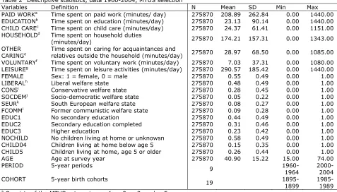
Besides age, period, and cohort, we distinguish a number of covariates. Time use is assumed to depend on sex, educational level, care for children under age 5, and welfare state. Table 2 presents the covariates and matching descriptive statistics.

2 _{This idea forms one of the pillars underlying life course policies introduced in the Netherlands and Belgium}

Table 2 Descriptive statistics, data 1960-2004, MTUS selection

Variables Definition N Mean SD Min Max

PAID WORKa

Time spent on paid work (minutes/ day) 275870 208.89 262.84 0.00 1440.00 EDUCATIONb _{Time spent on education (minutes/day) 275870 23.13 90.14 0.00 1440.00}

CHILD CAREc

Time spent on child care (minutes/day) 275870 24.37 61.41 0.00 1151.00 HOUSEHOLDd

Time spent on household duties

(minutes/day) 275870 174.21 157.31 0.00 1343.00 OTHER

CARINGe

Time spent on caring for acquaintances and

relatives outside the household (minutes/day) 275870 28.97 68.50 0.00 1085.00 VOLUNTARYf

Time spent on voluntary work (minutes/day) 275870 7.03 37.31 0.00 1080.00 LEISUREg

Time spent on leisure activities (minutes/day) 275870 290.57 185.42 0.00 1440.00 FEMALE Sex: 1 = female, 0 = male 275870 0.55 0.49 0.00 1.00 LIBERALh

Liberal welfare state 275870 0.48 0.49 0.00 1.00 CONSi _{Conservative welfare state 275870 0.28 0.45 0.00 1.00}

SOCDEMj

Socio-democratic welfare state 275870 0.05 0.22 0.00 1.00 SEURk

South European welfare state 275870 0.08 0.27 0.00 1.00 FCOMMl

Former communistic welfare state 275870 0.09 0.28 0.00 1.00 EDUC1 No secondary education 275870 0.44 0.49 0.00 1.00 EDUC2 Secondary education completed 275870 0.31 0.46 0.00 1.00 EDUC3 Higher education 275870 0.23 0.42 0.00 1.00 NOCHILD No children living at home or unknowsn 275870 0.58 0.49 0.00 1.00 CHILD04 Children living at home below age 5 275870 0.15 0.35 0.00 1.00 CHILD5 Children living at home, age 5 or older 275870 0.26 0.44 0.00 1.00 AGE Age at survey year 275870 40.90 15.22 15.00 74.00 PERIOD 5-year periods

9

1960-1964

2000-2004 COHORT 5-year birth cohorts

19

1895-1899

1985-1989

a

Consists of the MTUS categories: av1, av2, av3, and av5.

b _{Consists of the MTUS categories: av4 and av33.} c

Consists of the MTUS category: av11.

d

Consists of the MTUS categories: av6, av7, av9, av10, and av12.

e

Consists of the MTUS category: av8.

f

Consists of the MTUS category: av23.

g _{Consists of the MTUS categories: av17, av18, av19, av20, av21, av24, av25, av26, av27, av28, av29, av30, av31,}

av32, av34, av35, av36, av38, av39, and av40.

h

The following countries are assumed liberal welfare states: Canada, United States, United Kingdom, Australia, South Africa.

I

Conservative welfare states: France, the Netherlands, Belgium, Germany, West-Germany.

j

Socio-democratic welfare states: Denmark, Norway.

k

South-European welfare states: Italy.

l _{Former communist welfare states:Hungary, Poland, Czech Republic, East Germany, Yugoslavia, Slovenia.}

Source: MTUS-selection

4 . M ode l a n d r e su lt s

4 .1 Fix e d e ffe ct s m ode l

The structure of the age-period-cohort accounting/ multiple classification model / fixed-effects regression model can be written in linear regression form as

Y = Xb + ε, (1)

Where Y is a vector of event/ exposure rates or log-transformed rates from population tabular data, X is the regression design matrix consisting of “dummy variable” column vectors for the vector of model parameters b:

For i = 1, …, a age groups j = 1, …, p periods and μdenotes the intercept or adjusted mean rate;

αi denotes the ith row age effect or the coefficient for the ith age group; βj denotes the jthe

column period effect or the coefficient for the jth time period; γk denotes the kth diagonal cohort

effect or the coefficient for the kth cohort for k = 1, …, (a+p-1), with k = a-i+j; and εis a vector of random errors with mean 0 and constant diagonal variance matrix σ2I, where I is an identity matrix.

As mentioned in the introduction, the key problem in APC analysis using model (1) is the model identification problem. This problem arises in the conventional application of model (1) to tables of percentages or occurrence/exposure rates of events wherein age and period are of equal interval length in the population data and the diagonal cells in the age by period arrays represent the cohorts (see Yang & Land, 2006a).

Many studies focus on the “solution” of this problem. This literature has identified three conventional strategies for identification and estimation (see for more extensive overview Yang & Land, 2006a, p.83, Hagenaars, 1990 (in more general terms):

(1) constraining two or more of the remaining age, period, or cohort coefficients to be equal by placing at least one additional identifying constraint on the parameter vector; (2) using a “proxy” variable for the cohort or period effects and assuming that these variables are proportional to the selected dependent variables;

(3) changing at least one of the age, period, or cohort variables so that its relationship to the other age, period or cohort variables is nonlinear.

Taking into account these strategies, in particular the third mentioned, together with the hypothesis that there is a nonlinear age effect on time use, we specify and test a model of time use as a quadratic function of age.

i i i i i i i i i i i i i CHILD NOCHILD EDUC EDUC FCOMM SEUR SOCDEM CONS FEMALE AGE AGE PAIDWORK ε β β β β β β β β β β β β + + + + + + + + + + + + = 5 3

2 9 10 11

8 7 6 5 4 3 2 2 1

0 (3a)

i i i i i i i i i i i i i CHILD NOCHILD EDUC EDUC FCOMM SEUR SOCDEM CONS FEMALE AGE AGE EDUCATION ε β β β β β β β β β β β β + + + + + + + + + + + + = 5 3

2 _{9 10 11}

8 7 6 5 4 3 2 2 1

0 (3b)

i i i i i i i i i i i i i CHILD NOCHILD EDUC EDUC FCOMM SEUR SOCDEM CONS FEMALE AGE AGE CHILDCARE ε β β β β β β β β β β β β + + + + + + + + + + + + = 5 3

2 9 10 11

8 7 6 5 4 3 2 2 1

0 (3c)

i i i i i i i i i i i i i CHILD NOCHILD EDUC EDUC FCOMM SEUR SOCDEM CONS FEMALE AGE AGE HOUSEHOLD ε β β β β β β β β β β β β + + + + + + + + + + + + = 5 3

2 _{9 10 11}

8 7 6 5 4 3 2 2 1

0 (3d)

i i i i i i i i i i i i i CHILD NOCHILD EDUC EDUC FCOMM SEUR SOCDEM CONS FEMALE AGE AGE G OTHERCARIN ε β β β β β β β β β β β β + + + + + + + + + + + + = 5 3

2 _{9 10 11}

8 7 6 5 4 3 2 2 1

0 (3e)

i i i i i i i i i i i i i CHILD NOCHILD EDUC EDUC FCOMM SEUR SOCDEM CONS FEMALE AGE AGE VOLUNTARY ε β β β β β β β β β β β β + + + + + + + + + + + + = 5 3

2 9 10 11

8 7 6 5 4 3 2 2 1

0 (3f)

i i i i i i i i i i i i i CHILD NOCHILD EDUC EDUC FCOMM SEUR SOCDEM CONS FEMALE AGE AGE LEISURE ε β β β β β β β β β β β β + + + + + + + + + + + + = 5 3

2 _{9 10 11}

8 7 6 5 4 3 2 2 1

0 (3g)

for i = 1, 2, … ,N.

as fixed. This ignores the possibility that the effects of cohort and period may have random, as well as, or instead of, fixed effects on time use. Because of that respondents in the same cohort and / or period may be similar in their time use due to the fact that they share random error components unique to their cohorts or periods. The standard errors of estimated coefficients of conventional fixed-effects regression models may be underestimated. This heterogeneity problem can be addressed by modifying the fixed effects specification of the general APC regression model toward a random effects model (see Yang & Land, 2006a, 2006b). This implies that we should modify the fixed-effects APC regression model to a mixed effects model. For that purpose, we specify a mixed (fixed and random) effects APC regression model.

4 .2 Ra n dom e ffe ct s APC m ode l

In cross-sectional surveys such as MTUS, respondents are members simultaneously in cohorts and periods. Individuals are nested within cells created by the cross-classification of period and cohort. Table 3 shows this data structure.

Table 3 Two-way cross-classified data structure in MTUS: number of observations in each cohort-by-period cell Period

Cohort 1960-64

1965-69

1970-74

1975-79

1980-84

1985-89

1990-94

1995-99

2000-04

Total

1895-99 887 2 8 0 0 0 0 0 0 897

1900-04 0 96 12 495 0 0 0 0 0 603

1905-09 3128 1668 60 1082 216 0 0 0 0 6154 1910-14 0 1875 85 1201 705 606 0 0 0 4472 1915-19 0 231 529 1496 853 1682 736 0 0 5527 1920-24 0 4144 882 2412 1131 2344 3232 431 0 14576 1925-29 3767 220 867 2577 1067 3038 4073 1668 1421 18698 1930-34 0 5382 971 2464 1247 3234 4193 1787 2968 22246 1935-39 0 2512 1048 2492 1176 3629 4634 1665 3657 20813 1940-44 1451 1722 1073 2681 1581 4009 5759 1826 4124 24226 1945-49 0 70 1255 3397 2005 5017 5692 2478 5050 24964 1950-54 0 0 1043 2841 1855 5588 6573 2786 5931 26617 1955-59 0 0 0 2322 1897 5614 7479 3048 6337 26697 1960-64 0 0 0 418 1504 5019 7312 3156 6789 24198 1965-69 0 0 0 0 942 3465 5777 2785 6767 19736 1970-74 0 0 0 0 0 1518 5666 2348 6503 16035 1975-79 0 0 0 0 0 0 2661 1980 5586 10227

1980-84 0 0 0 0 0 0 0 1610 5322 6932

1985-89 0 0 0 0 0 0 0 0 2252 2252

Total 9233 17922 7833 25878 16179 44763 63787 27568 62707 275870 Source: MTUS

Each row is a birth cohort and each column is a period of 5 years. The number of birth cohorts is indicated as J and the number of periods as K. The numbers in this J by K matrix are the sample sizes, njk ; the numbers of individuals who belonged to a given birth cohort and were surveyed in

a given period.

A cross-classified effects APC model is estimated to assess the relative importance of the two contexts, cohort, and period, in understanding the individual differences in time use. Variability in time use (i.e. ‘paid work’, ‘education, training and schooling’, ‘care for children’, ‘household work’, ‘care for others’, ‘voluntary work’, and ‘leisure activities’, associated with individuals, cohorts, and periods in such a model is specified as follows:

ijk ijk ijk ijk ijk ijk ijk ijk ijk ijk ijk ijk jk ijk e CHILD NOCHILD EDUC EDUC FCOMM SEUR SOCDEM CONS FEMALE AGE AGE PAIDWORK + + + + + + + + + + + + = 5 3

2 9 10 11

8 7 6 5 4 3 2 2 1 0 β β β β β β β β β β β

β _(4a)

ijk ijk ijk ijk ijk ijk ijk ijk ijk ijk ijk ijk jk ijk e CHILD NOCHILD EDUC EDUC FCOMM SEUR SOCDEM CONS FEMALE AGE AGE EDUCATION + + + + + + + + + + + + = 5 3

2 _{9 10 11}

8 7 6 5 4 3 2 2 1 0 β β β β β β β β β β β

β _(4b)

ijk ijk ijk ijk ijk ijk ijk ijk ijk ijk ijk ijk jk ijk e CHILD NOCHILD EDUC EDUC FCOMM SEUR SOCDEM CONS FEMALE AGE AGE CHILDCARE + + + + + + + + + + + + = 5 3

2 _{9 10 11}

8 7 6 5 4 3 2 2 1 0 β β β β β β β β β β β

β _(4c)

ijk ijk ijk ijk ijk ijk ijk ijk ijk ijk ijk ijk jk ijk e CHILD NOCHILD EDUC EDUC FCOMM SEUR SOCDEM CONS FEMALE AGE AGE HOUSEHOLD + + + + + + + + + + + + = 5 3

2 9 10 11

8 7 6 5 4 3 2 2 1 0 β β β β β β β β β β β

β _(4d)

ijk ijk ijk ijk ijk ijk ijk ijk ijk ijk ijk ijk jk ijk e CHILD NOCHILD EDUC EDUC FCOMM SEUR SOCDEM CONS FEMALE AGE AGE G OTHERCARIN + + + + + + + + + + + + = 5 3

2 9 10 11

8 7 6 5 4 3 2 2 1 0 β β β β β β β β β β β

β _(4e)

ijk ijk ijk ijk ijk ijk ijk ijk ijk ijk ijk ijk jk ijk e CHILD NOCHILD EDUC EDUC FCOMM SEUR SOCDEM CONS FEMALE AGE AGE VOLUNTARY + + + + + + + + + + + + = 5 3

2 _{9 10 11}

8 7 6 5 4 3 2 2 1 0 β β β β β β β β β β β

β _(4f)

ijk ijk ijk ijk ijk ijk ijk ijk ijk ijk ijk ijk jk ijk e CHILD NOCHILD EDUC EDUC FCOMM SEUR SOCDEM CONS FEMALE AGE AGE LEISURE + + + + + + + + + + + + = 5 3

2 _{9 10 11}

8 7 6 5 4 3 2 2 1 0 β β β β β β β β β β β

β _(4g)

) , 0 ( ~ N

σ

Level-2 or “between-cell” model:

)

,

0

(

~

),

,

0

(

~

,

0 0 0

0jk

γ

u

v

u

N

τ

v

N

τ

β

=

+

+

Combined model: ijk k i ijk ijk ijk ijk ijk ijk ijk ijk ijk ijk ijk ijk e v u CHILD NOCHILD EDUC EDUC FCOMM SEUR SOCDEM CONS FEMALE AGE AGE TIMEUSE + + + + + + + + + + + + + + = 0 0 2 2 1 0 5 3 2 β β

γ _(4i)

for i = 1, 2, ..., njk individuals within cohort j and period k;

j = 1, …, 19 birth cohorts;

k = 1, …, 9 time periods;

where, within each birth cohort j and period k, respondent i’s time use is modeled as a function of his or her age, age-squared, educational attainment, gender, presence of young children, and welfare state. This random-intercepts model specification allows only the level-1 intercept to vary randomly from cohort-to-cohort and period-to-period, but not the level-1 slopes.

In this model, β0jk is the intercept or “cell mean” – that is, the mean time use of individuals who

belong to birth cohort j and surveyed in period k; β1, …. β11, are the level-1 fixed effects; eijk is

the random individual effect; the deviation of individual ijk‘s score from the cell mean; γ0 is the

model intercept, or grand-mean time use of all individuals; u0j is the residual random effect of cohort j that is, the contribution of cohort j averaged over all periods on β0jk, assumed normally distributed with mean 0 and variance τu ; and v0j is the residual random effect of period k; the

contribution of period k averaged over all cohorts, assumed normally distributed with mean 0 and variance τv . In addition, β0j = γ0 + u0j is the cohort effect averaged over all periods; and β0k =

4 .3 Re su lt s

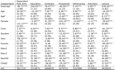
Tables 4 and 5 show the empirical estimates for regression models on the MTUS-data. Table 4 contains baseline ordinary least squares estimates of regression models without controls for period and cohort effects applied to 275870 respondents (equations 3). Estimates of various regression models, one for each time use category, are given in the table.

Table 4 Fixed-Effects Regression Models for Various Time Use Categories, MTUS Data, 1960-2004, Without Controls for Period and Cohort Effects

Dependent

Independent Paid work Education Childcare Household Othercaring Voluntary Leisure Intercept -89.71*** (3.88) 226.93*** (1.31) 79.47*** (0.84) -40.00*** (2.13) 5.15*** (1.10) 2.50*** (0.60) 478,35*** (2.82) Age 20.26*** (0.18) -10.16*** (0.06) 7.02*** (0.24) 6.26*** (0.10) 0.94*** (0.05) -0.70* (0,03) -10.29*** (0.13) Age2 -0.27*** (0.002) 0.10*** (0.001) 0.001 (0.000) -0.45*** (0.001) -0.005*** (0.001) 0.002*** (0.00) 0.13*** (0.002) Female -131.17*** (0.93) -3.30*** (0.32) 21.39*** (0.20) 144.15*** (0.51) -12.05*** (0.26) -1.11*** (0.14) -39.63*** (0.68) Cons 3.32*** (1.10) 5.54*** (0.38) 7.02*** (0.24) 6.37*** (0.61) 8.89*** (0.31) 2.49*** (0.17) -61.24*** (0.80) Socdem 5.49*** (2.08) 13.71*** (0.71) 3.19*** (0.45) -12.52*** (1.14) 3.47*** (0.58) -1.30*** (0.32) 2.92*** (1.51) Seur -68.10*** (1.75) 0.53 (0.59) -2.90*** 0.38) 35.04*** (0.96) -9.77*** (0.49) 1.39*** (0.27) -10.34*** (1.27) Fcomm 53.53*** (1.68) 5.83*** (0.57) -0.36 (0.36) 16.40*** (0.922) 2.89*** (0.47) 0.87** (0.26) -89.20*** (1.22) Educ2 13.95*** (1.10) -0.81* (0.37) 2.58*** (0.24) -14.56*** (0.60) 2.39*** (0.31) 2.80*** (0.17) 1.67* (0.80) Educ3 24.28*** (1.21) 11.81*** (0.41) 7.08*** (0.26) -21.48*** (0.67) 2.10*** (0.34) 5.70*** (0.19) -9.26*** (0.88) Nochild 53.53*** (1.51) 31.38*** (0.48) -83.65*** (0.31) -45.54*** (0.78) -2.39*** (0.40) 0.22 (0.22) 46.98*** (1.03) Child5 28.51*** (1.51) 24.44*** (0.51) -58.92*** (0.33) -18.18*** (0.83) -0.38 (0.42) 1.86*** (0.23) 27.53*** (1.10) AIC 3811125 3214975 2966670 3479721 3107680 2778052 3635020

Note: Standard errors are in parentheses;

*indicates p < 0.05; **indicates p < 0.01; ***indicates p < 0.001, two-tailed test.

Table 5 reports the parameter estimates for the crossed random effects model (equations 4) estimated on the MTUS data3. These results are attained using the restricted maximum-likelihood-empirical Bayes estimated method (Raudenbush and Bryk, 2002). Examining the fit statistics and information criteria at the bottom of the table, it can be seen that the AIC-values of the HAPC-models are lower than the AIC-values of the fixed-effect models (see table 3) which means that the HAPC-models fit the data better. The significant residuals in table 4 indicate that individual differences among the respondents remain after accounting for differences between cohorts and periods. The Intercept parameter is the variance in intercept across cohorts and periods. With a 1-tailed test at α = 0.05 there is evidence that intercepts (group means) do vary. These two estimates provide information for calculating the intraclass correlation, which determines the need for a higher level of analysis. The intraclass correlation (ρ) is the measure of differences between groups (cohorts, periods) relative to differences within groups4_{. High values}

means that the assumption of independence of errors is violated, and a hierarchical analysis is needed to avoid inflated Type I error rate. But, with large samples -as the MTUS sample is- even small values of ρ lead to inflated Type error I (see Tabachnick, 2005). Based on the significant Intercept parameters and the values of ρ, a need for higher order analyses can be seen.

The model estimates in Table 5 were estimated by SPSS PROC mixed.

4 ₂ 2 2 1 2 2 l l l

s

s

s

+

=

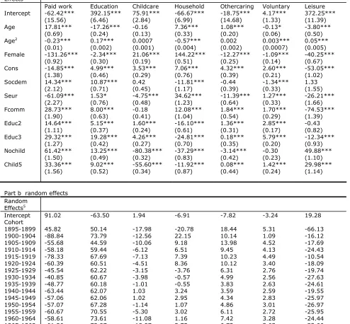
Table 5 HAPC Models for Various Time Use Categories, MTUS Data, 1960-2004

Part a fixed effects Fixed

Effects

Paid work Education Childcare Household Othercaring Voluntary Leisure Intercept -62.42*** (15.56) 392.15*** (6.46) 75.91*** (2.84) -66.67*** (6.99) -18.75*** (14.68) 4.17*** (1.33) 372.25*** (11.39) Age 17.81*** (0.69) -17.26*** (0.24) -0.16 (0.13) 7.36*** (0.33) 1.08*** (0.20) -0.13* (0.06) -3.80*** (0.50) Age2 -0.23*** (0.01) 0.17*** (0.002) 0.0007 (0.001) -0.57*** (0.004) 0.002 (0.002) 0.003*** (0.0007) 0.05*** (0.005) Female -131.26*** (0.92) -2.34*** (0.30) 21.06*** (0.19) 144.22*** (0.51) -12.27*** (0.25) -1.09*** (0.14) -40.25*** (0.67) Cons -14.85*** (1.38) 4.99*** (0.46) 3.53*** (0.29) 7.06*** (0.76) 4.32*** (0.39) 2.60*** (0.21) -53.05*** (1.02) Socdem 14.34*** (2.12) 10.87*** (0.71) 0.42 (0.45) -11.81*** (1.17) -0.44 (0.39) -1.34*** (0.33) 1.33 (1.55) Seur -61.09*** (2.27) 1.53* (0.76) -4.75*** (0.48) 34.62*** (1.23) -11.39*** (0.64) 1.27*** (0.33) -26.21*** (1.66) Fcomm 28.73*** (1.90) 8.00*** (0.63) -0.18 (0.41) 12.08*** (1.04) 1.84*** (0.54) 1.70*** (0.29) -74.53*** (1.39) Educ2 14.64*** (1.11) 5.15*** (0.37) 1.60*** (0.24) -16.10*** (0.61) 1.36*** (0.31) 2.85*** (0.17) -0.43 (0.82) Educ3 29.32*** (1.27) 19.28*** (0.42) 4.26*** (0.27) -24.81*** (0.70) 0.18*** (0.35) 5.79*** (0.20) -12.34*** (0.93) Nochild 61.42*** (1.50) 13.25*** (0.49) -80.38*** (0.32) -37.29*** (0.83) -3.14*** (0.42) -0.30 (0.23) 49.88*** (1.10) Child5 33.36*** (1.56) 9.02*** (0.52) -55.60*** (0.34) -11.92*** (0.87) 0.08*** (0.44) 1.42*** (0.24) 29.98*** (1.14)

Part b random effects Random

Effects5

Intercept 91.02 -63.50 1.94 -6.91 -7.82 -3.24 19.28

Cohort

1895-1899 45.82 50.14 -17.98 -20.78 18.44 5.31 -66.13 1900-1904 -88.84 73.79 -12.56 22.15 10.14 1.09 -16.12 1905-1909 -55.68 44.59 -10.06 9.18 13.98 4.52 -17.69 1910-1914 -58.18 59.44 -6.12 6.51 9.45 4.13 -24.43 1915-1919 -78.33 67.69 -7.13 7.39 10.23 4.49 -10.54 1920-1924 -60.39 60.51 -4.51 8.36 10.12 3.40 -18.09 1925-1929 -45.54 62.22 -3.15 -3.76 6.31 2.76 -19.74 1930-1934 -40.85 60.67 -3.98 -0.57 4.99 2.56 -27.63 1935-1939 -48.77 60.18 -1.01 -0.55 3.83 2.63 -24.61 1940-1944 -63.44 62.07 1.03 3.24 3.59 2.59 -19.55 1945-1949 -57.06 62.06 1.02 2.95 4.34 2.83 -25.97 1950-1954 -57.07 67.28 -1.14 1.07 4.86 3.01 -26.97 1955-1959 -60.67 70.55 -5.30 3.02 6.11 2.72 -25.95 1960-1964 -58.61 73.61 -11.08 1.16 7.42 3.28 -24.44 1965-1969 -61.96 72.07 -10.07 3.75 6.72 3.63 -22.66 1970-1974 -71.47 73.06 -3.56 7.89 7.27 3.03 -22.67 1975-1979 -37.21 47.80 0.51 0.31 8.47 3.35 -20.99 1980-1984 -6.39 19.75 3.44 1.86 5.83 3.23 -9.78

1985-1989 0 0 0 0 0 0 0

Period

1960-1964 -116.97 15.87 12.27 9.96 9.54 -0.71 35.55 1965-1969 -109.70 5.79 2.03 -4.94 2.51 1.44 32.95

5

1970-1974 -57.18 10.04 3.56 -7.49 14.00 2.79 13.87 1975-1979 -52.72 10.44 8.03 17.68 3.52 0.64 -5.92 1980-1984 -32.77 -10.63 0.80 7.98 3.30 -0.48 -15.38 1985-1989 -29.02 -1.71 1.61 2.69 3.21 0.33 -4.68 1990-1994 -42.46 -1.90 -0.84 11.72 -5.39 0.10 6.04 1995-1999 -25.29 -3.25 1.83 -5.34 9.53 -0.38 7.30

2000-2004 0 0 0 0 0 0 0

AIC 3803450 3193238 2961352 3477470 3105314 2777756 3632507

Covariance parameters

Residual 56822.10*** (153.03)

6217.19*** (16.74)

2684.85*** (7.23)

17437.84*** (46.96)

4522.00*** (12.18)

1380.75*** (3.72)

30577.11*** (82,35) Intercept 2537.49***

(387.26)

1278.07*** (185.14)

44.32*** (6.58)

240.47*** (36.30)

316.07*** (77.18)

4.21*** (0.79)

1350.57*** (236.00)

Ρ 0.043 0.17 0.016 0.014 0.065 0.0032 0,042

Note: Standard errors are in parentheses;

*indicates p < 0.05; **indicates p < 0.01; ***indicates p < 0.001, two-tailed test.

Examining the estimated average effect coefficients for cohorts, it can be seen that the estimated effects on time spent on paid work are particularly positive for the latest birth cohorts, and more negative for the earliest birth cohorts. Also the 1925-1929, 1930-1934, and 1935-1940 birth cohorts spend relatively much time on paid work. With respect to time spent on training and schooling, the various birth cohorts do not seem to differ much with the exception of the latest birth cohorts. The estimated effects on time spent on child care are particularly positive for the 1940-1944 and 1945-1949 cohorts, and the youngest birth cohorts. We also see a positive trend from the oldest birth cohorts to the 1940-1944 and 1945-1949 cohorts, and a negative trend on time spent on child care from the baby boom cohorts to the 1970-1974 cohort. The youngest birth cohorts seem to spend (again) more time on child care. The birth cohorts that appear to spend more time on paid work, spend less hours on household work than the other cohorts. With respect to time spent on care for others, we see a negative trend from the oldest birth cohort to the 1940-1944 cohort, and a positive trend from that cohort to the 1975-1979 birth cohort. The youngest birth cohorts appear to spend less time on care for others. With respect to voluntary work, no clear differences can be observed for the various birth cohorts. Time spent on that activity seem to be relatively constant over the various birth cohorts. Regarding time spent on free time, we see that the estimated effects are particularly positive for the youngest birth cohorts, and negative for the oldest.

seventies, and the end of the nineties than in the other periods. For the 1990-1994 period, the effect on time spent on care for others is particularly negative. The effects on time spent on voluntary work are particularly positive for the late sixties and early seventies. With respect to free time spending, the eighties seem to form a break-point as we see a clear negative trend from the early sixties to the early eighties, and a positive trend onwards.

Examining next the estimated individual-level coefficients in table 5 it can be seen that the qualitative results are quite similar to those given in table 4. The estimated regression coefficients and their standard errors are numerically quite similar between the two tables for the sex, education, and children variables. Estimates for the components of the quadratic age curve are quite different however. For instance, for the linear component of this curve, the estimated coefficient for time spent on child care is reduced from a highly significant 7.02 of table 4 to a nonsignificant -0.16 in table 5, after cohort and time period effects are taken into account. Also for time spent on leisure activities the coefficient for that term is reduced substantially, from -10.29 for the fixed effects model to -3.80 for the HAPC. For time spent on schooling and training the coefficient increased after cohort and period effects are included, from -10.16 to -17.26. The coefficients of the quadratic component of the age curve change also after cohort and period effects are taken into account. For instance for time spent on caring for others, the estimated coefficient increased from a significant -0.005 in table 4 to a nonsignificant 0.002 in table 5. For time spent on leisure activities, the coefficient decreased from 0.13 in table 4 to 0.05 in table 5. Besides the age-effects, also the estimated coefficients for welfare state are quite different for most activities, and change signs for some activities and welfare state types. These findings imply that a failure to control for the effects of cohort and period variation in time use could lead to substantial over- and underestimates of time use variations that are due to aging and also to substantial over- and underestimates of time use variations that are related to the welfare state people participate in.

5 . Con clu sion

Re fe r e n ce s

Anxo, D., J.Y. Boulin, C. Fagan, I. Cebrian, S. Keuzenkamp, U. Klammer, CH. Klenner, G. Moreno and L. Toharia (2006), Working time options over the life course: new work patterns and company strategies, European foundation for the improvement of living and working conditions, Dublin: EFILWC.

Becker, H.A. (1992), Generaties en hun kansen, Amsterdam: Meulenhoff.

Bovenberg, A.L. (2005), “Balancing work and family life during the life course”, De Economist, 153: 399-423

Easterlin, R.A. (1980), Birth and fortune: the impact of numbers on personal welfare, New York: Basic books.

Fu, W.J. (2008), “a Smooting cohort model in age period cohort analysis with applications to homicide arrest rates and lung cancer mortality rates”, Sociological methods & research, 36: 327-361.

Fu, W.J. (2000), “Ridge estimator in singular design with application to age-period-cohort analysis of disease rates”, Communications in statistics-theory and method, 29:263-278. Glenn, N.D. (1976), “Cohort analysts’ futile quest: statistical attempts to separate age, period,

and cohort effects”, American sociological review, 41:900-904.

Glenn, N.D. (2003), “Distinguishing age, period, and cohort effects”, in: J.T. Mortimer and M.J. Shanahan (eds.), Handbook of the life course, New York: Kluwer Academic/Plenum, 465-476. Hagenaars, J.A. (1990), Categorical longitudinal data: log-linear, panel, trend, and cohort

analysis, Newbury Park:: Sage Publications.

Hobcraft, J., J. Menken, and S. Preston (1982), “Age, period, and cohort effects in demography: a review”, Population index, 48:4-43.

Inglehart, R. (1977), The silent revolution: changing values and political styles among western publics, Princeton, NJ: Princeton University Press.

Inglehart, R. (1997), Modernization and postmodernization: cultural, economic and political change in 43 societies, Princeton, NJ: Princeton University Press.

Klammer, U., S. Keuzenkamp, I. Cebrian, C. Fagan, Ch. Klenner and G. Moreno (2005), Working time options over the life course: changing social security structures, European foundation for the improvement of living and working conditions, Dublin: EFILWC.

Kronjee, G.J. (1991), Veranderingen in levenscyclus, demografische veroudering en collectieve sociale uitgaven, Utrecht: ISOR/Universiy of Utrecht.

Liefbroer, A.C. and P.A. Dykstra (2000), Levenslopen in verandering, WRR voorstudies en achtergronden V107, Den Haag: Sdu Uitgevers.

Mulder, C.H. (1993), Migration dynamics: a life course approach, dissertation, Amsterdam: Thesis publishers.

Naegele, G., C. Barkholdt, B. de Vroom, J. Goul Andersen and K. Kramer (2003), A new organisation of time over working life, European foundation for the improvement of living and working conditions, Dublin: EFILWC.

O’Brien, R.M., K. Hudson, and J. Stockard (2008), “A mixed model estimation of age, period, and cohort effects”, Sociological methods & research, 36: 402-428.

O’Brien, R.M. (2000), “Age period cohort characteristic models”, Social science research, 29: 123-39.

Robertson, C., S. Gandini, and P. Boyle (1999), “Age-Period-Cohort models: a comparative study of available methodologies”, Journal of clinical epidemiology, 52:569-583.

Ryder, N.B. (1965), “The cohort as a concept in the study of social change”, American sociological review, 30:843-861.

Schmid, G. (2000), “Transitional Labour Markets. A New European Employment Strategy”, in: B. Marin, D. Meulders & D. Snower (eds.), Innovative Employment Initiatives, Aldershot, etc.: Ashgate, 223-253.

Schmid, G. and B. Gazier (2002), The Dynamics of Full Employment: Social Integration Through Transitional Labour Markets, Cheltenham, UK and Brookfield, US: Edward Elgar.

Tabachnick, B. G. (2005), Multilevel modeling with SPSS, workshop presented at Loyola Marymount University, Los Angeles, CA.

Versantvoort, M.C. (2000), Analysing labour supply in a life course perspective, dissertation, Amsterdam: Thela thesis.

Wilson, J.A. and W.R. Grove (1999), “The intercohort decline in verbal ability: does it exist?”,

American sociological review”, 64:253-266.

Yang, Y. and K.C. Land (2006a), “A mixed models approach to the age-period-cohort analysis of repeated cross-section surveys, with an application to data on trends in verbal test scores”,

Sociologcial methodology, 36:75-97.

Re se a r ch M e m or a n du m D e pa r t m e n t of Econ om ics

Research Memoranda

- are available from Department of Economics homepage at : http://www.economie.leidenuniv.nl - can be ordered at Leiden University, Department of Economics, P.O. Box 9520, 2300 RA Leiden, The

Netherlands Phone ++71 527 7756 / 7855; E-mail: [email protected]

2008.02 Maroesjka Versantvoort

Time use during the life course in USA, Norway and the Netherlands: a HAPC-analysis. 2008.01 Maroesjka Versantvoort

Studying time use variations in 18 countries applying a life course perspective. 2007.06 Olaf van Vliet

Globalisation, European Integration and Social Protection – Patterns of Change or Continuity? 2007.05 Ben van Velthoven

Kosten-batenanalyse van criminaliteitsbeleid. Over de methodiek in het algemeen en Nederlandse toepassingen in het bijzonder.

2007.04 Ben van Velthoven

Rechtseconomie tussen instrumentaliteit en normativiteit.

2007.03 Guido Suurmond

Compliance to fire safety regulation. The effects of the enforcement strategy. 2007.02 Maroesjka Versantvoort

Een schets van de sociaal-economische effecten van verlof en de beleidsmatige dilemma’s die daaruit volgen.

2007.01 Henk Nijboer

A Social Europe: Political Utopia or Efficient Economics? An assessment from a public economic approach.

2006.04 Aldo Spanjer

European gas regulation: A change of focus. 2006.03 Joop de Kort and Rilka Dragneva

Russia’s Role in Fostering the CIS Trade Regime. 2006.02 Ben van Velthoven

Incassoproblemen in het licht van de rechtspraak. 2006.01 Jurjen Kamphorst en Ben van Velthoven

De tweede feitelijke instantie in de belastingrechtspraak. 2005.03 Koen Caminada and Kees Goudswaard

Budgetary costs of tax facilities for pension savings: an empirical analysis. 2005.02 Henk Vording en Allard Lubbers

How to limit the budgetary impact of the European Court's tax decisions? 2005.01 Guido Suurmond en Ben van Velthoven

Een beginselplicht tot handhaving: liever regels dan discretionaire vrijheid. 2004.04 Ben van Velthoven en Marijke ter Voert

Paths to Justice in the Netherlands. Looking for signs of social exclusion.

2004.03 Guido Suurmond

Brandveiligheid in de horeca. Een economische analyse van de handhaving in een representatieve gemeente.

2004.01 Koen Caminada and Kees Goudswaard

Are public and private social expenditures complementary? 2003.01 Joop de Kort

De mythe van de globalisering. Mondialisering, regionalisering of gewoon internationale economie?

2002.04 Koen Caminada en Kees Goudswaard

Inkomensgevolgen van veranderingen in de arbeidsongeschiktheidsregelingen en het nabestaandenpensioen.

2002.03 Kees Goudswaard

Houdbare solidariteit. 2002.02 Ben van Velthoven

Civiele en administratieve rechtspleging in Nederland 1951-2000; deel 1: tijdreeksanalyse. 2002.01 Ben van Velthoven

Civiele en administratieve rechtspleging in Nederland 1951-2000; deel 2: tijdreeksdata. 2001.03 Koen Caminada and Kees Goudswaard

International Trends in Income Inequality and Social Policy. 2001.02 Peter Cornelisse and Kees Goudswaard

On the Convergence of Social Protection Systems in the European Union. 2001.01 Ben van Velthoven

De rechtsbijstandsubsidie onderzocht. En hoe nu verder? 2000.01 Koen Caminada

Pensioenopbouw via de derde pijler. Ontwikkeling, omvang en verdeling van premies lijfrenten volgens de Inkomensstatistiek.

1999.03 Koen Caminada and Kees Goudswaard

Social Policy and Income Distribution. An Empirical Analysis for the Netherlands.

1999.02 Koen Caminada

Aftrekpost eigen woning: wie profiteert in welke mate? Ontwikkeling, omvang en verdeling van de hypotheekrenteaftrek en de bijtelling fiscale huurwaarde.

1999.01 Ben van Velthoven and Peter van Wijck Legal cost insurance under risk-neutrality. 1998.02 Koen Caminada and Kees Goudswaard

Inkomensherverdeling door sociale zekerheid: de verdeling van uitkeringen en premieheffing in 1990 en 1995.

1998.01 Cees van Beers

Biased Estimates of Economic Integration Effects in the Trade Flow Equation. 1997.04 Koen Caminada and Kees Goudswaard

Distributional effects of a flat tax: an empirical analysis for the Netherlands. 1997.03 Ernst Verwaal

Compliance costs of intra-community business transactions. Magnitude, determinants and policy implications.

1997.02 Julia Lane, Jules Theeuwes and David Stevens

High and low earnings jobs: the fortunes of employers and workers. 1997.01 Marcel Kerkhofs and Maarten Lindeboom

Age related health dynamics and changes in labour and market status.

1996.07 Henk Vording

The case for equivalent taxation of social security benefits in Europe. 1996.06 Kees Goudswaard and Henk Vording

1996.05 Cees van Beers and Jeroen C.J.M. van den Bergh

The impact of environmental policy on trade flows: an empirical analysis. 1996.04 P.W. van Wijck en B.C.J. van Velthoven

Een economische analyse van het Amerikaanse en het continentale systeem van proceskostentoerekening.

1996.03 Arjan Heyma

Retirement and choice constraints: a dynamic programming approach. 1996.02 B.C.J. van Velthoven en P.W. van Wijck

De economie van civiele geschillen; rechtsbijstand versus no cure no pay. 1996.01 Jan Kees Winters

Unemployment in many-to-one matching models. 1995.05 Maarten Lindeboom and Marcel Kerkhofs

Time patterns of work and sickness absence. Unobserved effects in a multi-state duration model. 1995.04 Koen Caminada en Kees Goudswaard

De endogene ontwikkeling van de belastingdruk: een macro-analyse voor de periode 1960-1994.

1995.03 Henk Vording and Kees Goudswaard

Legal indexation of social security benefits: an international comparison of systems and their effects.

1995.02 Cees van Beers and Guido Biessen

Trade potential and structure of foreign trade: the case of Hungary and Poland. 1995.01 Isolde Woittiez and Jules Theeuwes

Well-being and labour market status.

1994.10 K.P. Goudswaard

Naar een beheersing van de Antilliaanse overheidsschuld. 1994.09 Kees P. Goudswaard, Philip R. de Jong and Victor Halberstadt

The realpolitik of social assistance: The Dutch experience in international comparison. 1994.08 Ben van Velthoven

De economie van misdaad en straf, een overzicht en evaluatie van de literatuur. 1994.07 Jules Theeuwes en Ben van Velthoven

De ontwikkeling van de criminaliteit in Nederland, 1950-1990: een economische analyse. 1994.06 Gerard J. van den Berg and Maarten Lindeboom

Durations in panel data subject to attrition: a note on estimation in the case of a stock sample. 1994.05 Marcel Kerkhofs and Maarten Lindeboom

Subjective health measures and state dependent reporting errors. 1994.04 Gerard J. van den Berg and Maarten Lindeboom

Attrition in panel data and the estimation of dynamic labor market models.

1994.03 Wim Groot

Wage and productivity effects of enterprise-related training.

1994.02 Wim Groot

Type specific returns to enterprise-related training. 1994.01 Marcel Kerkhofs