Modelling the dynamics of angles of human RR intervals

Modelling the dynamics of angles of human R–R

intervals

N.B. Janson†‡, A.G. Balanov†, V.S. Anishchenko‡, P.V.E. McClintock†

†Department of Physics, Lancaster University, Lancaster, LA1 4YB, UK

‡Department of Physics, Saratov State University, Astrakhanskaya 83, 410026, Saratov, Russia

PACS numbers: 05.45.Tp, 87.10+e, 87.19.Hh

Abstract.

Heart rate variability (HRV) data from young healthy humans is expanded into two components, namely, the angles and radii of a map of R–R intervals. It is shown that, for most subjects at rest breathing spontaneously, the map of successive angles reveals a highly deterministic structure after the frequency range below ∼ 0.05 Hz has been filtered out. However, no obvious low-dimensional structure is found in the map of successive radii. A recently proposed model describing the map of angles for a periodic self-oscillator under external periodic and quasiperiodic forcing is successfully applied to model the dynamics of such angles.

1. Introduction

Modelling the behaviour of real systems is often useful and almost always a challenge. Living systems, within which a large number of processes interact and mix in a complex way, while being influenced by different kinds of noise, are especially difficult to treat. There are several ways to attack the problem, including e.g. constructing a mock-up based on prior knowledge of principles governing the function of the system, or creating a virtual model. The method of modelling that we discuss below is somewhat different and consists of constructing a mathematical model in the form of an equation describing the evolution of the system’s state in time. We apply this approach to the human cardiovascular system. We focus on the well-known phenomenon of heart rate variability (HRV), which manifests itself in the fact that successive R–R intervals extracted from an electrocardiogramme usually differ.

There has been a long-running debate among researchers applying the tools of time series analysis to HRV data as to the nature of this variability, considered from the viewpoint of nonlinear dynamics. The central question has been whether R–R intervals can be attributed to a certain deterministic process perturbed by noise, or it is rather due to some random fluctuation for which only probabilistic laws are valid. Obviously, any natural process derives from a complex mixture of deterministic and stochastic factors. Therefore, the above question is actually reduced to the question which of the components, stochastic or deterministic, dominates. A desirable ambition could be also to reveal the concrete sources of determinism and stochasticity.

Since variation of R–R intervals is far from being regular, for a long time the phenomenon was attributed to some kind of random process. Conventional statistical methods were applied to characterize it, including e.g. Fourier power spectra, autocorrelation functions, mean value and variance. Later, the discovery of the phenomenon of dynamical chaos in 1976 [1], led to the fascinating suggestion that the behaviour of many complex physiological signals like the ECG (and consequently HRV as well) [2] may be explicable in terms of chaotic dynamics, that is, they can be described by deterministic equations of motion, perhaps influenced by noise. However, further studies seemed to contradict this idea [3, 4], and revealed that HRV possesses many features in common with stochastic rather than deterministic processes, e.g. a 1/fα

a satisfactory description of the observed dynamics as control parameters were changed. All the models mentioned above attempted to capture the behavior of the R–R intervals themselves, without expanding them into any components. In spite of some degree of success, none of the models were able to reproduce reliably the full set of basic HRV properties. In [13], however, attention was paid to anangular component of the R–R intervals map in humans undergoing paced respiration at a frequency close to 0.1 Hz, and distinct structure was found in the angles map. So, it was concluded that determinism occured in HRV duringpaced respiration. However, it was inferred that the “complexity ofspontaneousrespiratory movements obviouslyprecludesthe identification of finite-dimensional attractors in heart rate fluctuations within the frequency range of breathing”. An empirical model in the form of one-dimensional autonomous map was suggested to describe approximately the behaviour of the angles of the R–R intervals map, possessing, however, a piecewise-linear return function that is non-smooth (non-differentiable at several points), which does not seem a very natural way of modelling real processes.

In the present paper we demonstrate that removal from human R–R intervals of the frequency range below ∼0.05 Hz, measured at rest with spontaneousbreathing, allows obviously deterministic structure to be revealed in the map of angles. We also model the behaviour of the angles with the help of a map that was previously derived for the case of weakly interacting periodic oscillators [14]. We show that only the angles of the R–R intervals map exhibit highly deterministic behaviour, whereas the corresponding radii reveal no obvious low-dimensional structure either before or after filtration. Finally, we discuss the results obtained.

2. Description of the model.

It is known that several oscillatory processes are involved in the dynamics of the cardiovascular system, each of them having a characteristic timescale (period). There are, for example, heart contraction, respiration, and myogenic activity of smooth muscles. Obviously, all these processes interact with each other, and their interaction is reflected in the Fourier and wavelet spectra of many known cardiovascular signals [15], including the ECG, where several characteristic peaks can be detected.

From the viewpoint of oscillation theory, the interaction of m periodic processes gives rise to quasiperiodic motion (in general), which can be represented as an m -dimensional torus in the state space of a dynamical system. The same torus can be also modelled by applying one or several external periodic driving forces to a system with purely periodic oscillations. An illustration of how a two-dimensional torus is formed is given in Fig. 1. In this case, if the interacting periodic processes are not synchronous, the trajectory fills the whole torus surface and is never closed. If they are synchronous, the trajectory lying on the torus surface is closed after one or several windings.

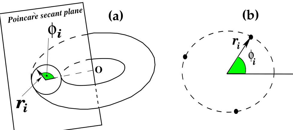
a nontrivial task. To simplify consideration, a Poincar´e map is often introduced [16] as follows (Fig. 2(a) illustrates the simplest case of a two-dimensional torus): a surface is selected in such a way that it intersects all of the system’s trajectories transversely (at a nonzero angle, i.e. does not touch them). The points of intersection in only one direction are selected strictly preserving their order in time, to form the Poincar´e map. Such a map contains the complete dynamical information about the motion in the original system except information about the real time, since instead of the original continous time t only discrete time i is available. A Poincar´e map of a two-dimensional torus is in general a closed curve, often called a “circle”. If two periodic processes interact and are not synchronized, the map points fill the whole circle. If they are synchronized, the map consists of a finite number of points lying on this circle. In Fig. 2(b) a Poincar´e map is shown for the synchronous case consisting of three points on a circle shown by dashed line and being the section of the torus surface.

An alternative type of discrete data can also be used which, unlike Poincar´e maps, preserve information about the real time of the system, namely, return times. The return times of the system are defined as the time intervals between the trajectory’s intersection in one direction with the secant plane. One can also obtain return times in an easier way from a one-dimensional signal coming from the system under study by defining some threshold and taking the time intervals between successive crossings of it by the signal in one direction (for example, from above to below), as in Fig. 1(c). An example of return times which is well-known in physiology are the R–R intervals extracted from a human ECG, as illustrated by Fig. 3.

It is known that a map of successive return times is qualitatively similar to the Poincar´e map of the system under study [17], provided that the latter is deterministic, i.e. that its changes of state can be described by some evolution equations. A famous example of such a map in physiology is the scattergramme obtained from R–R intervals. Let us consider a return times map of a typical dynamical system within which two periodic processes interact weakly. We can define an angle φi and a radius ri for

every point of the map as shown in Fig. 2(b). If the processes are synchronous, one will observe a discrete set of map points, and, consequently, a discrete set of possible values of angles φi. If the processes are not synchronous, the angles φi will be allowed to take

any value within [−π:π].

In [14] a model was derived for the dynamics of angles of return times map of a periodic self-oscillatory system forced by an arbitrary number of harmonic signals. We now give a brief description of how it was derived.

Consider a periodic self-oscillator whose natural oscillations (in the absence of any forcings) are of frequency ω0 and amplitude R. If the nonlinearity in the oscillator is weak then, in the absence of forcings, as time tends to infinity, its signal can be approximated by a sinusoidal function of time, and its oscillations correspond in phase space to a closed loop (Fig. 1(a)). Now let the oscillator be forced by a sinusoidal signal with frequency Ω and amplitude r (Fig. 1(b)). If the forcing is weak, r R, a signal

terms: one sine term describing oscillations with frequency ω and amplitude R and a second sine term describing oscillations with the frequency of the external forcing Ω and its amplitude r (Fig. 1(c)), that is:

x(t) =Rsinωt+rsin Ωt, r R. (1)

As a result of the forcing a two-dimensional torus is born (Fig. 1(c), right). A well-known phenomenon which can take place in forced periodic oscillators, as well as in mutually coupled oscillators, is synchronization. This means that forcing (or coupling) can change the frequency of oscillations in the system so that it is no longer equal to the natural frequency and appears to be related to the frequency of forcing (or to the frequency of the coupled oscillator) as integer numbers. To quantify the interaction between two oscillators a rotation number is introduced, defined as the ratio of their frequencies during interaction. This number can be rational or irrational§. If it is rational and equals n

m, then one can say that n

m synchronization is taking place.

Thus, the frequency ωin (1) coincides with the natural frequencyω0 in the absence of synchronization. In the presence of synchronization, it is shifted in the direction defined by the forcing. If the oscillations are synchronized by the forcing, the rotation number of the whole system under consideration, here denoted as ξ = Ω

ω, is equal to n m,

where n, m are integers.

The return times of our system are defined as the time intervals between successive crossings by the signal x(t) of the threshold x = 0 in one direction (Fig. 1(c)). After some calculations, the return times are obtained explicitly using the fact that the forcing is weak (details are given in [14]). After that, the map of return times is introduced, the origin is placed at the centre of mass of the map, and the angles φi are defined as

shown in Fig. 2(b). Finally, the explicit map describing the dynamics of angles for weak harmonic forcing is found to take the simple form:

φi = arctan (2 cos 2πξ−cotφi−1). (2)

Similarly, for any numbernof sinusoidal forcings with different frequencies Ωj and small

amplitudes Aj (j = 1, . . . , n) the signal x(t) coming from the forced oscillator can be

approximated by:

x(t) =Rsinωt+

n

X

j=1

Ajsin Ωjt, Aj R (3)

and the following map for angles is obtained:

§ A number is rational, if it can be represented as a fraction of two integer numbersn andm, i.e. n m,

φi = arctan{2 cos Θ1−cotφi−1

+ 2[

n

X

j=2

βjcos (iΘj+

Θj

2 )(cos Θj−cos Θ1)]

× [

n

X

j=1

βjcos (iΘj +

Θj

2 )]

−1

} (4)

βj =

Aj

A1

sin (Θj/2)

sin (Θ1/2)

, β1 = 1.

Here, Θj = 2πξj, while ξj =

Ωj

ω defines the “partial” rotation number. For two forcing

signals, the formulae take the form:

φi = arctan{2 cos Θ1−cotφi−1+ 2β2[ cos Θ2−cos Θ1]×

× [β2 +

cos(iΘ1+Θ₂1) cos (iΘ2+Θ₂2)

]−1

}, β2 =

A2

A1 sinΘ2

2 sinΘ1

2

. (5)

All the above maps (2), (4) and (5) are defined via the arctan function which varies between [−π

2;

π

2]. However, it is obvious that the angles φi are defined in such a way that they will vary within [−π;π]. To resolve this contradiction, we redefine the right-hand sides of our equation in such a way, that for all positive argumentsφi−1 we preserve

their values, and for all negative ones we deduct π. In terms of their physical meaning all the above maps are circle maps [18, 19, 20], (2) being autonomous, and (4) and (5) being non-autonomous (meaning that the right-hand side depends explicitly on discrete time i). We will follow the traditional representation by plotting all such maps, both theoretical and experimental, within a square with the limits [−π:π].

Numerical simulations show that, provided the interaction is weak, the maps for angles of return times either for the forced oscillator or for coupled oscillators fit closely the theoretically predicted maps (2) or (5) for either two or three processes involved, respectively. Some examples of how the map (5), describing interaction between three

processes, looks are illustrated in Fig. 4. Let us define that process whose amplitude is largest in the given one-dimensional dataset as the main rhythm, and denote its frequency as ω.

In Figs. 4 (a) and (b) the frequencies of forcing signals are selected to be irrationally connected with the basic frequency ω = 1 and with each other in order to show what the maps look like in the absence of any synchronization. Fig. 4(a) shows a map for the case of forcing with a frequency Ω1 = 0.1012032011. . . (a random sequence of 0,1,2,3 after ”0.1”) at relatively large amplitude A1 = 0.1, while the second forcing with frequency Ω2 = 0.3102130202. . . (a random sequence of 0,1,2,3 after ”0.3”) has a smaller amplitudeA2 = 0.012. The whole map is concentrated within the vicinity of the one-dimensional curve defining the return functionk of (2) forξ = Ω

ω = 0.1012032011. . .

(grey line). Thus, the appearance of the map for angles gives an immediate idea of the approximate frequency ratio of the dominant processes. One can see that the points in this example fill the whole allowed space densely, though with different probability, and that no one-dimensional structures can be observed. This is due to the absence of any synchronization between the processes involved.

In Fig. 4(b) a map is given for the case when interaction between the process with frequency Ω1 = 0.3102130202. . . (a random sequence of 0,1,2,3 after “0.3”) has a relatively large amplitude A1 = 0.2, while the process with frequency Ω2 = 0.1012032011. . . (a random sequence of 0,1,2,3 after ”0.1”) has the smaller amplitude

A2 = 0.1. The situation is the same as in Fig. 4(a), apart from the fact that the interaction of the main rhythm with the process of frequency Ω1 now prevails, and the map lies in the vicinity of the return function of (2) with ξ = 0.3102130202. . . (grey line).

Figs. 4 (c) and (d) illustrate what happens when only two out of the three processes are synchronous. For Fig. 4(c) the two rhythms with smaller amplitudes are synchronized with each other and neither is synchronous with the main rhythm. The value of ω is chosen to be 1.0103210. . . (a random sequence of 0,1,2,3 after ”1.”). Ω1 = 0.1 and Ω2 = 0.2, A1 = 0.1,A2 = 0.11. One observes two one-dimensional curves pointing explicitly to the existence of synchronization between the two minor rhythms. The grey line shows the return function of (2) for ξ= 0.2.

In Fig. 4(d) synchronization between the main rhythm and one of the minor rhythms occurs. Here, ω = 1, Ω1 = 1₃, Ω2 = 0.2103021. . . (a random sequence of 0,1,2,3 after ”0.2”),A1 = 0.2,A2 = 0.1. The existence of synchronisation between the main rhythm and the process with Ω1 is revealed by the presence of three closed loops in the angles map. The number of closed loops gives the denominator 3 of the corresponding rotation numberξ1 = 1₃; the loops can be seen to lie on the return function of (2) forξ= 1₃ (grey line).

3. Dynamics of angles of human R–R intervals

3.1. Data description

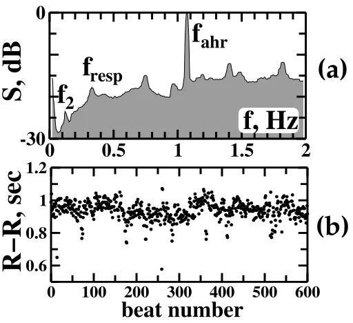
As is widely appreciated, the Fourier spectrum of an ECG measured for a healthy human (Fig. 5) contains several distinct peaks at different frequencies, namely, the main peak at the average heart rate fahr, a peak of smaller amplitude associated with respiration

as x(t) = Pδ(t − ti) and subjected to almost analytical calculation of the Fourier

transform. This method allows one to obtain an approximation of the Fourier spectrum of the actual ECG that produced the given R–R intervals, with the real frequencies on the abscissa axis. Note that the main component, corresponding to basic heart rhythm, is then present in the spectrum. In addition to the peaks, as mentioned in Introduction, a 1/fα _{(“one-over-f”) behaviour of the Fourier power spectrum is observed in the range}

of super-low frequencies below ∼0.005 Hz. The existence of several spectral peaks is in itself often taken as evidence for the presence of several processes interacting within the single system. Following this hypothesis, let us apply the technique of plotting the map for angles, extracted from the map of successive R–R intervals, to study the interactions between different processes.

3.2. Data pre-processing

As shown in Section 2, the shape of the map for angles is largely determined by the ratio of the frequencies of the processes whose interaction is the strongest compared to their interaction with other processes. Usually, in the R–R intervals of healthy people one observes a very slow but noticeable floating of the average value (Fig. 5(b)). It is related to the very low frequencies mentioned above, which are much less than the average heart rate and thus lead to a rotation number close to zero. The map of angles extracted from the map of original R–R intervals (Fig. 6, upper row) thus reveals this floating immediately . The effect was important in all the datasets which we consider in this paper, and the whole map lies in the vicinity of the return function of (2) for the value of ξ = 0 (grey line). Over small observation times, of the order of minutes, this floating can be regarded as nonstationarity. In order to consider as stationary motion as possible, and to focus on interactions of the main heart rhythm with respiration and the process of frequency ∼ 0.1 Hz, it is therefore reasonable to try to filter out the corresponding frequency range, that is, the range below ∼0.05 Hz.

For this purpose we use two methods of filtering in this paper. Denote a discrete sequence of R–R intervals as x(i). The first method consists of computing the analogue of the second derivative of the original time series x(i):

xder(i) =

x(i+ 1) +x(i−1)−2x(i)

2 . (6)

We will refer to this procedure as the method of derivatives. The second method is slightly more intricate and consists of the following procedure: (i) we find all the local maximaxmax(j) and minimaxmin(j) of the time seriesx(i); and (ii) each datapointx(i) located between the j-th local maximum xmax(j) and the jth local minimum xmin(j), or between thejth_{minimum and the (j+1)}th_{maximum, including the extrema themselves,} is replaced by a new value xdiff(i)

xdiff(i) = x(i)− 1

2(xmax(j)−xmin(j)), or

xdiff(i) = x(i)− 1

respectively. Thus, the filter (7) simply deducts from every datapoint the local average, and in what follows we will call this technique the method of differences.

The results of applying these two filters are slightly different and we compute the power spectrum for every filtered data set xder or xdiff in order to control the effect of filtering. To compute the Fourier spectrum from filtered R–R intervals we just add to

xder orxdiff the average value of unfiltered R–R intervals, and then proceed in the same way as for original, non-filtered data [21]. In Fig. 6 (middle row) the results of filtering by means of derivatives are given, while Fig. 6 (lower row) illustrates the workability of the differences technique. The methods of differences and derivatives both remove the trend from the data. However, the noisy background of the Fourier power spectrum seems on average to be more uniform after filtration by derivatives, than by differences, although the use of derivatives leads to a significant decrease of the lower-frequency range (around 0.1 Hz and less). In both cases, all three dominating frequencies and their combinations are clearly seen after filtration, but the ratios of their amplitudes appear to be slightly different.

Extract the angles φi from the maps of filtered R–R intervals and plot the map for

angles (Fig. 6, middle and lower rows). The two ways of filtering appear to result in somewhat different behaviours of the angles φi. For the case considered, both angles

maps seem to lie in the vicinity of the same curve, but points are placed with some phase shift. The differences method leads to a more smeared map, while that of derivatives reveals the structure better. In Fig. 6 (middle and lower rows) the points of both the filtered angles maps lie close to the one-dimensional continuous curve that represents the return function of map (2) forξ = 1

3 which is shown by the grey line. They seem to be formed by three fairly isolated clouds of points, thus testifying to the presence of 1₃ synchronization between heart rate and the most dominant of the other processes (which in the present case seems to be respiration). For further analysis we select whichever filter leads to the more pronounced structure in the map for angles. Of course, neither of the filtration techniques described is perfect, and other techniques might be used instead to obtain similar or perhaps even better results.

Several typical examples of angles maps arising in filtered human R–R intervals are shown in Figs. 7 and 8. All the datasets were obtained in the course of measurements undertaken to study the possibility of synchronizing the human heart rate by means of weak external periodic forcing in the form of a sequence of sound and light pulses. The light pulse was a red square appearing on the screen of a computer for 0.1 sec, and the sound was generated by the computer speakers and had the same duration. The frequency of the sound was 440 Hz, corresponding to the musical note “la”. The sound was weak enough not to cause noticeable changes in heart rate and blood pressure. Two kinds of forcing were studied, namely: (i) a periodic sequence of pulses with a frequency close to, but slightly differing from, the average heart rate of the given subject at rest; and (ii) a sequence of pulses whosecurrentperiod was equal to thecurrentR–R interval

of another subject at rest. Each dataset was measured over an interval of 5 minutes

Hz. Details of the experiment and the results were presented in [22], where the forcing signals were compared with response signals by means of phase difference computations as in [23].

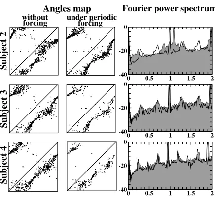
Here we present the results of processing of the same data using our new technique. Note that we study only the intrinsic structure of each HRV signal, and its change in response to forcing, without comparing it to any other signals. In Fig. 7 the plots in the 1st column are the angles maps extracted from filtered R–R intervals of subjects without forcing. The plots in the 2nd column are the angles maps for the same subjects under periodic forcing at a frequency being 1 per cent smaller than the average heart rate of the subject without forcing. The third column shows Fourier power spectra for the same subject without forcing (shaded) and under forcing (solid line). As one can see from the spectra, the main peak shifts to the left as a result of the forcing in each case.

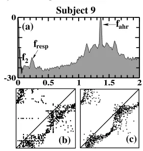
In Fig. 8 the plots in the 1st column are the angles maps of unforced subjects (different from those in Fig. 7), while the plots in the 2nd column are the angles maps of the same subjects under aperiodic forcing defined by the R–R intervals of another person. As in Fig. 7, the third column shows Fourier power spectra for the same subject without forcing (shaded) and under forcing (solid line). One can see that, in each case, a distinct structure is revealed in the angles maps. One can make the following observations:

(i) In spite of its weakness, the forcing can cause a noticeable change in the structure of angles map pointing to the changes in the ratio of interacting dominating frequencies (subjects 2, 4, 5, 6). Since the shape of the angles maps is mainly defined by interaction between the main heart rhythm and respiration, we can conclude that it is mainly the ratio of their frequencies that is changed under forcing.

(ii) In some subjects the angles map reveals several distinct clouds of points, which constitute evidence of synchronization between the main heart rhythm and respiration (in subject 1, 3 clouds; in subject 2 at rest, 5 clouds, and under forcing 3 clouds; in subject 3 under forcing, 3 clouds; in subject 4 under forcing, 4 clouds; in subject 7 both at rest and under forcing, 3 clouds). In many cases the appearance of these clouds is caused by the external forcing.

This apparently implies that even such a weak forcing generally increases the strength of interaction between the main heart rhythm and respiration, resulting in their synchronization.

(iii) Many experimental angles maps can be quite accurately approximated by the theoretically derived models (2) or (5) (actually, for all subjects except those mentioned below in item (iv)).

theoretical models (2) or (5), although they possess a pronounced structure (see subject 4 under forcing, and subject 7).

This means that, in some healthy subjects, the interaction of respiration with the main heart rhythm is relatively strong, an inference that is supported by the presence of second harmonics of the respiration frequency fresp in the Fourier spectrum (it is clearly seen in subject 4, but is much less pronounced in subject 7).

Unlike the angles φi of R–R intervals, the radii ri which are extracted from the

same data do not reveal any obvious low-dimensional structure, at least in their two-dimensional map. An example of a radii map is presented in Fig. 9, for which the radii

ri were extracted from R–R intervals of subject 2 under periodic forcing. The radii

obtained from either original (a) or filtered (b), (c) R–R intervals do not display any obvious deterministic behaviour, although the corresponding angles are highly regular (see Fig. 7, upper row).

3.3. Data Modeling

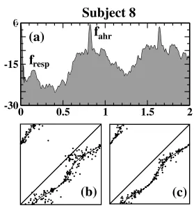
Let us illustrate how the maps (2) or (5) can model the angles of filtered human R–R intervals. In Fig. 10 an analysis of healthy human HRV data is illustrated, following filtration by the differences technique. Fig. 10(a) shows the Fourier power spectrum of a filtered dataset. It contains two distinct frequencies atfahr ≈0.82 Hz andfresp≈0.16 Hz. Points of angles map (Fig. 10(b)) are placed around a curve defining the return function of map (2) for ξ = 0.2 (thin solid line). Moreover, one can observe 5 clouds of points lying on this curve, testifying to the presence of 1

5 synchronization between the main heart rhythm and respiration. Note that the rotation number ξ = 1

5 defining synchronization differs slightly from the actual ratio of fresp and fahr, in full agreement with the theory of effective phase synchronization [25].

Now let us try to reproduce this map by means of modelling. Because there are basically two processes involved in the interaction, we choose map (2). Note, that the resulting dynamics of this map does not depend on the values of frequencies independently, but only on their ratio. For example, the valuesω = 1.4 and Ω = 0.7 will give the same result asω= 1 and Ω = 0.5 because their ratioξ= Ω

ω is the same. Bearing

this fact in mind, we select the following set of parameters: ω= 1, Ω1 = 0.2 (to obtain the rotation number ξ1 = 1₅). To simulate a real situation let us assume that random noise influences the value of respiration frequency and let its variance be 0.19. Let us also add a random term being Gaussian white noise to the right-hand part of equation (2) with variance 0.01. Iteration of the obtained map and removal of a transient process gives the phase portrait shown in Fig. 10(c). It looks very similar to the experimental angles map in Fig. 10(b).

(like in Fig. 4(c)) can be distinguished in the angles map (Fig. 11(b)), so it seems that neither of the processes involved is synchronized with the other. Since there are three basic processes involved in the interaction here, we choose the map (5) as a model. Set the parameter values as follows: frequencies ω = 1, Ω1 = 0.18 and Ω2 = 0.074, and amplitudes A1 = 0.1 and A2 = 0.05. Let noise modulate most of the parameters of the model as follows: the values of frequencies Ω1 and Ω2 with intensities 0.43, the values of amplitudes A1 with intensity 0.41 and A2 with intensity 0.05. Let also add to the right-hand part of equation noise with intensity 0.1. The phase portrait of the resulting map, shown in Fig. 11(c), looks remarkably similar to the experimental results shown in Fig. 11(b).

4. Discussion and Conclusion.

It seems that the theoretically obtained maps (2) and (5) are able to model successfully the angular part of R–R intervals from healthy humans, provided that contributions from the frequency range below ∼0.05 Hz are first removed by filtration.

The possibility of modelling the behaviour of experimental human R–R intervals that we have demonstrated is interesting, not only in itself, but also because it contributes to the long-term discussion about the fundamental nature of human heart rate variability. The fact that the angular component of experimental R–R intervals can be successfully modelled by a dynamical system serves as a strong argument for the deterministic nature of the interactions between the processes governing heart rate variability. regular (periodic or is in there radial component of R–R intervals does not exhibit any obvious low-dimensional determinism. Thus, we can distinguish between two separate components of heart rate variability – one that displays highly regular behaviour, and one that does not display any obvious regularity at all.

5. Acknowledgements

The authors are grateful to N.B. Igosheva and G.V. Bordyugov for the assistance in data measurements. The work was supported by the Engineering and Physical Sciences Research Council (UK), the Medical Research Council (UK) and the U.S. Civilian Research Development Foundation (award No. REC 006).

References

[1] E.M. Lorenz 1963J. Atmos. Sci.20130

[2] A. Babloyantz, A. Destexhe 1988Biol. Cybern. 58203

[3] J.K. Kanters, N.H. Holstein – Rathlou, E. Agner 1994J. Cardiovascular Electrophysiology 5(7) 591

[4] K.H. Chon, J.K. Kanters, R.J. Cohen, N.-H. Holstein-Rathlou 1997Physica D99471 [5] M. Kobayashi, T. Musha 1982IEEE Transaction of Biomedical Engineer29456

[7] N. Iyengar, C.-K. Peng, R. Morin, A.L. Goldberger, L.A. Lipsitz 1996Am. J. of Physiology40(9) R1078

[8] A. Potapov 1988 In: Nonlinear Analysis of Physiological Data, Ed. H. Kantz, J. Kurths, and G. Mayer-Kress (Springer, Berlin) 117

[9] H. Kantz, T. Shreiber 1988IEE Proceedings – Science, Measurement and Technology145(6) 279 [10] M. Rosenblum and J. Kurths 1995Physica A215(4) 439

[11] H. Seidel, H. Herzel 1998Physica D115145

[12] P.Ch. Ivanov, L.A. Nunes Amaral, A.L. Goldberger, H.E. Stanley 1998Europhysics Letters43363 [13] K. Suder, F.R. Drepper, M. Schiek and H.-H. Abel 1998Modeling in Physiology44H1092 [14] N.B. Janson, A.G. Balanov, V.S. Anishchenko, P.V.E. McClintock 2001Phys. Rev. Lett861749 [15] A. Stefanovska and M. Bra˘ci˘c 1999Contemporary Physics4031

[16] N.V. Butenin, Yu.I. Neimark, N.A. Fufaev 1987 Introduction in theory of nonlinear oscillations

(Moscow: Nauka, in Russian)

[17] T. Sauer 1994 Phys. Rev. Lett. 72 3811; Janson N.B., Pavlov A.N., Neiman A.B., Anishchenko V.S. 1998Phys. Rev. E58R4

[18] V.I. Arnol’d 1983Geometrical Methods in the Theory of Ordinary Differential Equations (Springer-Verlag, New York)

[19] J. Guckenheimer and P. Holmes 1983Nonlinear Oscillations(Springer-Verlag, New York) [20] L. Glass 1991Chaos 113

[21] R.W. DeBoer, J.M. Karemaker, J. Strackee 1984IEEE Trans. on Biomed. Eng.31(4) 384 [22] V.S. Anishchenko, A.G. Balanov, N.B. Janson, N.B. Igosheva, G.V. Bordyugov 2000 Int. Jour.

Bifurcation & Chaos10(10) 2339

[23] M.G. Rosenblum, A. Pikovsky and J. Kurths 1996Phys. Rev. Lett.761804;

t

_i

t

_i+1

external sinusoidal forcing

resulting forced oscillations

(c)

(b)

(a)

periodic self−oscillations

x

0

Poincare secant plane

φ

i

i

r

O

φ

r

_i

i

(a)

(b)

Figure 2. (a) Surface of a two-dimensional torus and the way how Poincar´e map is constructed. (b) Poincar´e map (or a return times map which is qualitatively the same) for a two-dimensional torus for 1:3 synchronization. φi is the instantaneous angle, and

riis the instantaneous radius. Dashed line indicates the section of the two-dimensional

torus surface.

0

1

2

time, sec

ECG

Q

_S

P

T

R

_{R−R interval}

Partial synchronization

between two of three processes

No synchronization

between any two of three processes

(a)

(b)

(d)

(c)

Figure 4. Four examples of how the theoretical map (5) describing the interaction of three processes behaves for different parameter values. (a), (b), no synchronization between the processes. (c), (d), partial synchronization between two of the three processes involved. Details are given in text.

0 100 200 300 400 500 600 0.6

0.8 1

1.2

0

0.5

1

1.5

2

-30

0

f

_ahr

resp

f

f

₂

f, Hz

beat number

R−R, sec

S, dB

(a)

(b)

Figure 5. (a) A typical Fourier power spectrum computed for a sequence of R–R intervals. fahris the average heart rate,fresp is the respiration frequency, andf2is the

0

0.5

1

1.5

2

-40

-10

0 0.5 1 1.5 2

-30 0

0 0.5 1 1.5 2

-30 0

No filtering

by derivatives

Filtering

by differences

Filtering

Fourier power spectrum

Angles map

f

f

f

f

f

f

f

f

_f

Subject 1

(b)

(c)

(a)

Figure 6. Fourier power spectra and angles maps for R–R intervals of one subject (a) without any filtration; (b) after filtration by derivatives; (c) after filtration by differences. The grey lines indicate the return functions of map (2) for rotation number (a)ξ= 0 (b), (c)ξ = 1

0

0.5

1

1.5

2

-40

-20

0

0

0.5

1

1.5

2

-40

-20

0

0

0.5

1

1.5

2

-40

-20

0

Subject 2

Subject 3

Subject 4

Angles map

under periodic

forcing

forcing

without

Fourier power spectrum

Figure 7. Angles maps and Fourier power spectra from R–R intervals of humans in two different states: without forcing and under forcing. Each row illustrates a different subject. 1st column: map at rest, without forcing. 2nd column: map underperiodic

0 0.5 1 1.5 2 -40

-20 0

0 0.5 1 1.5 2 -40

-20 0

0 0.5 1 1.5 2 -40

-20 0

Subject 5

Subject 6

Subject 7

Angles map

Fourier power spectrum

forcing

forcing

without

under aperiodic

Figure 8. Angles maps and Fourier power spectra from R–R intervals of the same human in two different states: without forcing and under forcing. Each row illustrates a different subject. 1st column: map at rest, without forcing. 2nd column: map under

aperiodicforcing whose current period is defined by an R–R interval of another subject. 3rd column: Fourier power spectra of unforced R–R intervals (shaded) and forced ones (solid line).

(a)

(b)

(c)

Figure 9. Map of instantaneous radiiri extracted from the R–R intervals of subject 2

0

0.5

1

1.5

2

-30

-15

0

2.2 2.2 2.2 2.2 2.2 2.2 2.2

(a)

Subject 8

(b)

(c)

ahr

f

f

resp

0

0.5

1

1.5

2

-30

0

(a)

(b)

(c)

Subject 9

f

resp

f

₂

ahr

f