Munich Personal RePEc Archive
Exponential Spectral Risk Measures
Cotter, John and Dowd, Kevin
University College Dublin
2007
Online at
https://mpra.ub.uni-muenchen.de/3499/
Exponential Spectral Risk Measures
By
Kevin Dowd and John Cotter*
Abstract
Spectral risk measures are attractive risk measures as they allow the user to obtain
risk measures that reflect their subjective risk-aversion. This paper examines
spectral risk measures based on an exponential utility function, and finds that
these risk measures have nice intuitive properties. It also discusses how they can
be estimated using numerical quadrature methods, and how confidence intervals
for them can be estimated using a parametric bootstrap. Illustrative results suggest
that estimated exponential spectral risk measures obtained using such methods are
quite precise in the presence of normally distributed losses.
Keywords: spectral risk measures, risk aversion functions, exponential utility
function, parametric bootstrap
JEL Classification: G15
March 20, 2007
*
1. Introduction
One of the most interesting and potentially most promising recent developments
in the financial risk area has been the theory of spectral financial risk measures
(SRMs), recently proposed by Acerbi (2002, 2004). SRMs belong to the family of
coherent risk measures proposed by Artzner et alia (1997, 1999), and therefore
possess the highly desirable property of subadditivity1. It is also well-known by
now that the most widely used risk measure, the Value-at-risk (VaR), is not
subadditive, and the work by Artnzer et alia and Acerbi has shown that many (if
not most) of the inadequacies of VaR as a risk measure can be traced to its
non-subadditivity.
One of the nice features of SRMs is that they relate the risk measure itself
to the user’s subjective risk-aversion – in effect, the spectral risk measure is a
weighted average of the quantiles of a loss distribution, the weights of which
depend on the user’s risk-aversion function. Spectral risk measures enable us to
link the risk measure to the user’s attitude towards risk, the underlying objective
being to ensure that if a user is more risk averse, other things being equal, then
that user should face a higher subjective risk, which is what the SRM measures.
This means, for example, that two different investors might have the same
portfolios and share the same set of forecasts, but their subjective risk measures
will still be different if one of them is more risk averse than the other.
In principle, SRMs can be applied to any problems involving risky
decision making. Amongst many other possible applications, Acerbi (2004)
suggests that they can be used to set capital requirements or obtain optimal
risk-expected return tradeoffs in portfolio analysis, and Cotter and Dowd (2006)
suggest that SRMs could be used by futures clearinghouses to set margin
requirements that reflect their corporate risk appetites.
This paper investigates SRMs further. In particular, it focuses on SRMs
based on an underlying exponential utility function. Our objective is two-fold.
1
First, we seek to establish some of the properties of SRMs to see how intuitive
and ‘well-behaved’ they might be. Our second objective is computational: we
discuss how these SRMs might be estimated and also discuss how we might
estimate confidence intervals for them.
The article is organised as follows. Section 2 sets out the essence of
Acerbi’s theory of spectral risk measures. Section 3 discusses SRMs based on
exponential utility functions. Section 4 discusses the estimation of SRMs and
section 5 discusses the estimation of confidence intervals for them. Section 6
concludes.
2. Spectral Risk Measures
Following Acerbi (2004), consider a risk measure Mφ defined by:
(1) =
1
0
) (p q dp
Mφ φ p
where qp is the p loss quantile and φ(p) is a user-defined weighting aversion
function with weights defined over p, where p is a continuous range of cumulative
probabilities p∈[0,1]. We can think of Mφ as the class of quantile-based risk
measures, where each individual risk measure is defined by its own particular
weighting function.
Two well-known members of this class are the VaR and the Expected
Shortfall (ES). The VaR at the α confidence level is:
(2) VaRα =qα
The VaR places all its weight on a single quantile that corresponds to a chosen
confidence level, and places no weight on any others, i.e., with the VaR risk
measure, φ(p) takes the degenerate form of a Dirac delta function that gives the
For its part, the ES at the confidence level α is the average of the worst
α
−
1 of losses and (in the case of a continuous loss distribution) is:
(3) − = 1 1 1 α α
α q dp
ES p
With the ES, φ(p) gives tail quantiles a fixed weight of
α
− 1
1
and gives non-tail
quantiles weight of zero.
A drawback with both of these risk measures is that they inconsistent with
risk aversion in the traditional sense. This can be illustrated in the context of the
theory of lower partial moments (see Bawa (1975), Fishburn (1977) and
Grootveld and Hallerbach (2004)). Given a set of returns r and a target return
*
r , the lower partial moment of order k ≥0 around r* is equal to
} ] * , 0
{[max( r r k
E − . The parameter k reflects the user’s degree of risk aversion,
and the user is risk-averse if k >1, risk-neutral if k =1 and risk-loving if
1
0<k < . It can then be shown that the VaR is a preferred risk measure only if
0 =
k , i.e., the VaR is our preferred risk measure only if we are very risk-loving!
The ES would be our preferred risk measure if k =1, and this tells us that the ES
is our preferred risk measure only if the user is risk-neutral between better and
worse tail outcomes.
A user who is risk averse might prefer to work with a risk measure that
take account of his/her risk aversion, and this takes us to the class of spectral risk
measures (SRMs). In loose terms, an SRM is a quantile-based risk measure that
takes the form of (1) where φ(p) reflects the user’s degree of risk aversion. More
precisely, we can consider SRMs as the subset of Mφ that satisfy the following
properties of positivity, normalisation and increasingness due originally to
Acerbi:2
2
1. Positivity: φ(p)≥0.
2. Normalisation: =
1
0
1 ) (p dp
φ .
3. Increasingness: φ′(p)≥0.
The first coherent condition requires that the weights are weakly positive and the
second requires that the probability-weighted weights should sum to 1, but the
key condition is the third one. This condition is a direct reflection of
risk-aversion, and requires that the weights attached to higher losses should be no less
than the weights attached to lower losses. Typically, we would also expect the
weight φ(p) to rise with p.3 In a ‘well-defined’ case, we would expect the
weights to rise smoothly, and the more risk-averse the user, the more rapidly we
would expect the weights to rise.
A risk measure that satisfies these properties is attractive not only because
it takes account of user risk-aversion, but also because such a risk measure is
known to be coherent.4
However, there still remains the question of how to specify φ(p), and
perhaps the most natural way to obtain φ(p) is from the user’s utility function5.
3. Exponential Spectral Risk Measures
This requires us to specify the utility function, and a common choice is the
exponential utility function. This utility function is defined conditional on a single
parameter, the coefficient of absolute risk aversion. The exponential utility
function is defined as follows over outcomes x:
(4) U(x)=−e−ax
3
The conditions set out allow for the degenerate limiting case where the weights are flat for all p values, and such a situation implies risk-neutrality and is therefore inconsistent with risk-aversion. However, we shall rule out this limiting case by imposing the additional (and in the circumstances very reasonable) condition that φ(p) must rise over at least point as p increases from 0 to 1. 4
The coherence of SRMs follows from Acerbi (2004, Proposition 3.4). 5
where a>0 is the Arrow-Pratt coefficient of absolute risk aversion (ARA). The
coefficients of absolute and relative risk aversion are:
(5a) a x U
x U x
RA =
′ ′′ − = ) ( ) ( ) (
(5b) xa x U x U x x
RR =
′ ′′ − = ) ( ) ( ) (
We now set
(6) φ(p)=λe−a(1−p)
where λ is an unknown positive constant. This clearly satisfies properties 1 and
3, and we can easily show (by integrating φ(p) from 0 to 1, setting the integral to
1 and solving for λ) that it satisfies property 2 if we set
(7) a
e a − − = 1 λ
Hence, substituting (7) into (6) gives us the exponential weighting function (or
risk-aversion function) corresponding to (4):6
(8) a
p a e ae p − − − − = 1 ) ( ) 1 ( φ
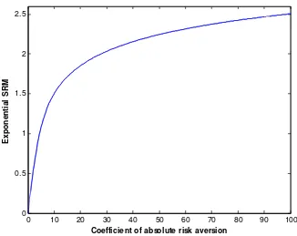
This risk-aversion function is illustrated in Figure 1 for two alternative values of
the ARA coefficient, a. Observe that this weighting function has a nice shape: for
the higher p values associated with higher losses, we get bigger weights for
greater degrees of risk-aversion. In addition, as p rises, the rate of increase of
) (p
φ rises with the degree of risk-aversion.
6
Insert Figure 1 here
The SRM based on this risk-aversion function, the exponential SRM, is
then found by substituting (8) into (1), viz.:7
(9) =
1
0
) (p q dp
Mφ φ p = − −
−
− =
1
0 ) 1 (
1 e e q dp
a
Mφ a a p p
We also find that the risk measure itself rises with the degree of
risk-aversion, and some illustrative results are given in Table 1. For example, if losses
are distributed as standard normal and we set a=5, then the spectral risk measure
is 1.0816. But if we increase a to 25, the measure rises to 1.9549: the greater the
risk-aversion, the higher the exponential spectral risk measure.
Insert Table 1 here
The relationship of the exponential SRM and the coefficient of absolute
risk aversion is illustrated further in Figure 2. We can see that the risk measure
rises smoothly as the coefficient of risk aversion increases, as we would expect.
Insert Figure 2 here
These results suggest that ESRMs are ‘well-behaved’ and have nice intuitive
properties.
4. Estimating Spectral Risk Measures
7
Estimates of (9) were obtained using Simpson’s rule numerical quadrature with p divided into
The equation for the SRM, (9), indicates that solving for the SRM involves
integration. Special cases aside, this integration would need to be carried out
numerically rather than analytically. This means that the estimation of SRMs
requires a suitable numerical integration or numerical quadrature method. Such
methods estimate the integral from a numerical estimate of its discretised
equivalent in which p is broken into a large number of N ‘slices’.8 This, in turn,
raises the question of how different quadrature methods compare. Furthermore,
since quadrature methods depend on a specified value of N, it also raises the issue
of how estimates might depend on the value of N.
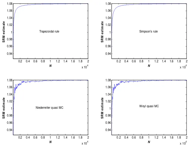
To investigate these issues further, Figure 3 provides some plots showing
how estimates of standard normal SRMs vary with different quadrature methods
and different values of N. These plots are based on an illustrative ARA coefficient
equal to 5, but we get similar plots for other values of this coefficient. The
methods examined are those based on the trapezoidal rule, Simpson’s rule, and
Niederreiter and Weyl quasi-Monte Carlo. As we might expect, all four
quadrature methods give estimates that converge on their true values as N gets
larger. However, the trapezoidal and Simpson’s rule methods produce estimates
that converge smoothly as N gets larger, whereas the two quasi-Monte Carlo
methods produce estimates that converge more erratically as N gets larger. The
plots also suggest that the first two methods are usually more accurate for any
given value of N, and that the method based on Simpon’s rule is marginally better
than that based on the trapezoidal rule.
Insert Figure 3 here
In addition, these plots show that all methods produce estimates of SRMs
that have a small downward bias. If we wish to get accurate estimates of SRMs, it
is therefore important to choose N value large enough to make this bias negligible.
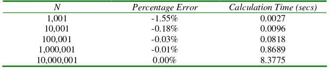
To investigate further, Table 2 reports results for the accuracy and calculation
times of the same SRM estimated using Simpson’s rule and different values of N.
This shows that, for N=1,001, we get an estimate with an error of -1.55% and this
8
takes 0.0027 seconds to calculate using the latest version (version 2007a) of
MATLAB using a Pentium 4 desktop computer. For N=10,001, the error is
-0.18% and this estimate takes 0.0096 seconds to calculate. The accuracy and
calculation times increase as N gets larger, and when N=10,000,001, we get an
error of -0.00% and a calculation time of a little over 8 seconds. Bearing in mind
that real-world risk measurement is subject to many different sources of error that
are beyond the control of the risk manager, it is pointless to go for spuriously
accurate estimates that ignore these other sources of error. We would therefore
suggest that a value of N=10,001 is for practical purposes accurate enough for the
needs of risk managers in the real world.9
Insert Table 2 here
5. Estimating Confidence Intervals for Spectral Risk Measures
Given that our estimates are prone to many sources of error, it is good practice to
estimate some precision metrics to go with our estimated risk measures, and
perhaps the best such metrics are estimates of their confidence intervals.
We can easily obtain such estimates using a parametric bootstrap, and this
can be implemented using the following procedure:
• Given N, for each of b bootstrap trials, we simulate a set of N loss values
from our assumed distribution, in this case a standard normal. We order
these simulated losses from lowest to highest to obtain a set of simulated
quantiles, q~ . We then apply our chosen quadrature method to (9) with p qp
replaced by q~ to obtain a bootstrap estimate of the SRM. p
• We repeat this step b times and obtain an estimate of the confidence interval
from the distribution of simulated SRM estimates.
9
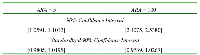
Some illustrative results are shown in Table 3. This shows estimates of the
90% confidence intervals for values of the ARA coefficient equal to 5 and 100.
The Table also shows estimates of the standardised confidence intervals, which
are equal to the 90% confidence intervals with the bounds divided by the mean of
the bootstrap SRM estimates. All results are based on N=10,001 and b=1000. We
can see that for ARA=5, the 90% confidence is [1.0591, 1.1012] and its
equivalent for ARA=100 is [2.4075, 2.5380]. For ARA=5, the standardised
interval is [0.9805, 1.0195] and for ARA=100 the standardised interval is [0.9739,
1.0267]. It is striking how narrow these intervals are: for ARA=5, the width of the
interval is only 3% of the estimated mean SRM, and for ARA=100, the width is
only a little over 5% of the estimated mean SRM. These narrow confidence
intervals indicate that the SRM estimates are very precise.
Insert Table 3 here
6. Conclusions
This paper has examined spectral risk measures based on an exponential utility
function. We find that the exponential utility function leads to risk-aversion
functions and spectral risk measures with intuitive and nicely behaved properties.
These exponential SRMs are easy to estimate using numerical quadrature methods
and accurate estimates can be obtained very quickly in real time. It is also easy to
estimate confidence intervals for these SRMs using a parametric bootstrap.
Illustrative results suggest that these confidence intervals are surprisingly narrow,
and this indicates that SRM estimates are quite precise. Of course, the results
presented here are based on an assumed normal distribution, and further work is
needed to establish results for other distributions.10
10
References
Acerbi, C., (2002) “Spectral Measures of Risk: A Coherent Representation of
Subjective Risk Aversion.” Journal of Banking and Finance, 26, 1505-1518.
Acerbi, C., (2004) “Coherent Representations of Subjective Risk Aversion.” Pp.
147-207 in G. Szegö (Ed.) Risk Measures for the 21st Century, New York:
Wiley.
Artzner, P., F. Delbaen, J.-M. Eber, and D. Heath, (1997) “Thinking coherently.”
Risk, 10 (November), 68-71.
Artzner, P., F. Delbaen, J.-M. Eber, and D. Heath, (1999) “Coherent Measures of
Risk.” Mathematical Finance, 9, 203-228.
Bawa, V. S., (1975) “Optimal Rules for Ordering Uncertain Prospects.” Journal
of Financial Economics, 2, 95-121.
Borse, G. J. (1997) Numerical Methods with MATLAB: A Resource for Scientists
and Engineers. Boston: PWS Publishing Company.
Bertsimas, D., G. J. Lauprete, and A. Samarov, (2004) “Shortfall as a Risk
Measure: Properties, Optimization and Applications.” Journal of Economic
Dynamics and Control, 28, 1353 – 1381.
Cotter, J., and K. Dowd, (2006) “Extreme Spectral Risk Measures: An
Application to Futures Clearinghouse Margin Requirements.” Journal of
Banking and Finance, 30, 3469-3485.
Dowd, K., (2005) Measuring Market Risk. Second edition, Chichester: John
Wiley and Sons.
Fishburn, P. C., (1977) Mean-Risk Analysis with Risk Associated with
Below-Target Returns.” American Economic Review, 67, 116-126.
Grootveld, H., and W. G. Hallerbach, (2004) “Upgrading Value-at-Risk from
Diagnostic Metric to Decision Variable: A Wise Thing to Do?” Pp. 33-50 in
G. Szegö (Ed.) Risk Measures for the 21st Century, Wiley, New York.
Kreyszig, E. (1999) Advanced Engineering Mathematics. 8th edition. Wiley, New
York.
Miranda, M. J., and P. L. Fackler, (2002) Applied Computational Economics and
FIGURES
Figure 1: Exponential Risk Aversion Functions
Figure 2: Plot of Exponential Spectral Risk Measure Against the Coefficient
of Absolute Risk Aversion: Standard Normal Loss Distribution
0 10 20 30 40 50 60 70 80 90 100
0 0.5 1 1.5 2 2.5
Coefficient of absolute risk aversion
E
x
p
o
n
e
n
ti
a
l
S
R
M
Figure 3: Estimates of Standard Normal Spectral Risk Measure for Various
Numerical Quadrature Methods and Values of N: Coefficient of Absolute
Risk Aversion = 5
0.2 0.4 0.6 0.8 1 1.2 1.4 1.6 1.8 2
x 104 0.94 0.96 0.98 1 1.02 1.04 1.06 1.08 S R M e s ti m a te Trapezoidal rule N
0.2 0.4 0.6 0.8 1 1.2 1.4 1.6 1.8 2
x 104 0.94 0.96 0.98 1 1.02 1.04 1.06 1.08 S R M e s ti m a te Simpson's rule N
0.2 0.4 0.6 0.8 1 1.2 1.4 1.6 1.8 2
x 104 0.94 0.96 0.98 1 1.02 1.04 1.06 1.08 S R M e s ti m a te
Niederreiter quasi MC
N
0.2 0.4 0.6 0.8 1 1.2 1.4 1.6 1.8 2
x 104 0.94 0.96 0.98 1 1.02 1.04 1.06 1.08 S R M e s ti m a te
Weyl quasi MC
N
Table 1: Values of Exponential Spectral Risk Measure with Standard Normal Losses
Coefficient of Absolute Risk Aversion
Exponential Spectral Risk Measure
1 0.2781
5 1.0816
25 1.9549
100 2.5055
Notes: Estimates are of (9) obtained using Simpson’s rule numerical quadrature with p divided into N=10,000,001 ‘slices’. The calculations were carried out using the Miranda-Fackler (2002) CompEcon functions in the 2007a version of MATLAB on a Pentium 4 desktop computer.
Table 2: Percentage Errors and Calculation Times for Estimates of Standard
Normal Exponential Spectral Risk Measure Obtained Using Simpson’s Rule:
Coefficient of Absolute Risk Aversion = 5
N Percentage Error Calculation Time (secs)
1,001 -1.55% 0.0027
10,001 -0.18% 0.0096
100,001 -0.03% 0.0818
1,000,001 -0.01% 0.8689
10,000,001 0.00% 8.3775
[image:16.612.133.471.398.468.2]Table 3: Illustrative Estimates of 90% Confidence Intervals for Spectral Risk
Measures
ARA = 5 ARA = 100
90% Confidence Interval
[1.0591, 1.1012] [2.4075, 2.5380]
Standardized 90% Confidence Interval
[0.9805, 1.0195] [0.9739, 1.0267]
Note: Estimates are of (9) obtained using Simpson’s rule numerical quadrature with