Modeling of Soft Tissues Interacting with Fluid (Blood or Air) Using the Immersed Finite Element Method

(1)

Modeling of Soft Tissues Interacting with Fluid (Blood or

Air) Using the Immersed Finite Element Method

Lucy T. Zhang

JEC 2049, Department of Mechanical, Aerospace, and Nuclear Engineering, Troy, USA Email: [email protected]

Received 26 November 2013; revised 30 December 2013; accepted 7 January 2014

Copyright © 2014 Lucy T. Zhang. This is an open access article distributed under the Creative Commons Attribution License, which permits unrestricted use, distribution, and reproduction in any medium, provided the original work is properly cited. In accordance of the Creative Commons Attribution License all Copyrights © 2014 are reserved for SCIRP and the owner of the intellectual property Lucy T. Zhang. All Copyright © 2014 are guarded by law and by SCIRP as a guardian.

ABSTRACT

This paper presents some biomedical applications that involve fluid-structure interactions which are si- mulated using the Immersed Finite Element Method (IFEM). Here, we first review the original and en- hanced IFEM methods that are suitable to model in- compressible or compressible fluid that can have den- sities that are significantly lower than the solid, such as air. Then, three biomedical applications are studi- ed using the IFEM. Each of the applications may re-quire a specific set of IFEM formulation for its re- spective numerical stability and accuracy due to the disparities between the fluid and the solid. We show that these biomedical applications require a fully-cou- pled and stable numerical technique in order to pro- duce meaningful results.

KEYWORDS

Biomechanics; Fluid-Structure Interactions; Biomechanics

1. INTRODUCTION

In the past decade, the interest in developing novel simulation techniques for modeling fluid-structure interactions revived due to the increasing demands in capabili- ties to accurately and efficiently study biomedical applications. Biomedical applications often involve fluid (blood) interacting with soft tissues. In some cases, the fluid can also be air, which has a disparate density compared to the soft tissues.

Since soft tissues come in with all forms, shapes and sizes, it is more convenient to set up a simulation using non-boundary-fitted modeling technique. The non-boundary-fitted approaches avoid the re-meshing process by defining independent meshes for the fluid and solid re-

spectively. The solid can freely move on top of the fluid grid without deforming the surrounding fluid. A widely used numerical approach for bio-interface applications is the immersed boundary (IB) method, which was initially proposed by Peskin to study the blood flow around heart valves [1-7]. The mathematical formulation of the IB method employs a mixture of Eulerian and Lagrangian descriptions for fluid and solid domains. In particular, the entire fluid domain is represented by a uniform background grid, which can be solved by finite difference method with periodic boundary conditions; whereas the submerged structure is represented by a fiber or boundary network. The interaction between the fluid and structure is accomplished by distributing the nodal forces and in- terpolating the velocities between Eulerian and Lagran- gian domains through a smoothed approximation of the Dirac delta function. The advantage of the IB method is that the fluid-structure interface is tracked automatically by following the displaced structural boundary movement, which removes the costly computations due to various mesh update algorithms. Many other numerical algorithms have been developed that are inspired by the IB method, such as the immersed interface method (IIM) [8-14], the extended immersed boundary method (EIBM) [15] and the immersed boundary finite element method (IB-FEM) [16,17]. A review on several methods can be found in [18].

(2)

this problem by representing the background viscous fluid with an unstructured finite element mesh and non-linear finite elements for the immersed deformable solid. Similar to the immersed boundary method, the fluid domain is defined on a fixed Eulerian grid. However, the solid domain is constructed independently with a La- grangian mesh, which makes it possible to use a more detailed constitutive model to describe the solid material such as linear elastic, hyperelastic and viscoelastic. This approach is particularly attractive to modeling biomedical applications including stent deployment, blood flow in athersclerosis in arteries, etc. [23-31]. With finite element formulations for both fluid and solid domains, the submerged structure is solved more realistically and accurately in comparison with the corresponding fiber network representation in the IB method. The caveat, of course, is to remove the artificial fluid where the solid volume occupies. Since the solid moves at every time step, the artificial fluid also moves. Using the non-boundary-fitted approach, this volume can be easily identified. The fluid solver is based on a stabilized equal-order finite element formulation applicable to problems involv- ing moving boundaries [32-34]. This stabilized formulation prevents numerical oscillations without introducing excessive numerical dissipations. It is also possible to assign sufficiently refined fluid mesh in local regions wherever necessary to obtain more accurate interfacial solutions.

The two-way coupled approach, i.e. the interpolation and the distribution of the velocity and the forces between the two domains, is quite robust when the solid be- haves very much like the fluid. However, if there exists high discontinuity in density as well as other intrinsic parameters in the solid and the fluid, the force and the ve-locity to be interpolated between the two fields can no longer provide consistent convergence. Therefore, a semi-implicit algorithm for the immersed finite element [35] was developed to alleviate the situations when large density difference and/or stiff solid material are used in the solid domain. The calculation of the fluid-structure interaction force is modified in order to achieve a larger stabilization range.

The semi-implicit IFEM algorithm works well when the fluid dominates the dynamics of the system, in which the solid moves and deforms by following the fluid flow. However, when the solid dynamics or inertia must be taken into account, letting the solid follow the fluid movement may lead to unrealistic solid deformation and sometimes even causes the distortion of the solid mesh, because it is not appropriate to still approximate the solid behaviors using only the fluid velocity. A modified IFEM algorithm (mIFEM) [36] was then introduced to provide a more accurate prediction of the solid motion and deformation, which directly depend on the solid inertia effects,

constitutive laws, and the fluid solutions near the fluid- structure interface. The results show that it produces more accurate and reasonable solid responses compared to the original IFEM algorithm.

In this paper, we first provide a detailed derivation and descriptions of the mathematical formulations for IFEM, the semi-implicit IFEM, and the modified IFEM. Then, we will show several biomedical applications that used IFEM algorithms. The choice of the algorithm used for each application is dependent on the nature of the fluid- structure interactions involved, which comes clear as the readers go through the motivations of each of the algorithm development.

2. KINEMATICS AND ASSUMPTIONS

2.1. Kinematics

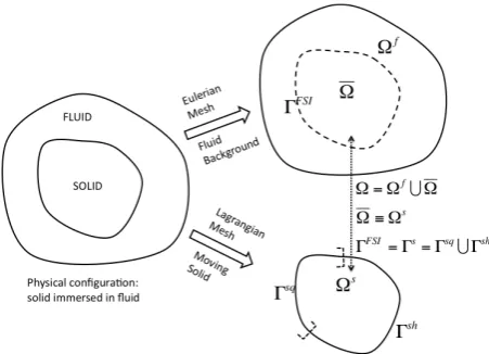
Let us consider a deformable structure that occupies a finite domain, Ωs, which is completely immersed in a fluid domain Ωf, as illustrated in Figure 1. The fluid and the solid together occupy the entire computational domain Ω, and they intersect at a common interface

FSI

Γ , where “FSI” represents a line if Ω is a two-dimensional domain or a surface if Ω is in three-dimensions. The interface ΓFSI coincides with the solid boundary Γs. The nomenclature involved can be partitioned into two categories: one belongs to the solid and the other to the fluid. The notations associated with the solid have superscript s to distinguish them from those of the fluid f.

2.2. Assumptions

Before showing derivations, we first need to state three assumptions:

1) The fluid exists everywhere in the domain, Ω. This assumption allows us to generate fluid and solid meshes and solve fluid and solid equations independently, thus avoiding frequent mesh updating schemes required to track the fluid-structure interface. In the IFEM, the solid immersed in the fluid domain occupies a physical space or volume in the computational domain. Therefore, when the solid domain, Ωs, is constructed, it overlaps with the entire domain Ω filled with fluid. Since both the solid and the “artificial” fluid co-exist in Ωs, it is also re- ferred to as the “overlapping domain”, Ω, i.e., Ω = Ωs , in later text. This is illustrated in Figure 1. This assumption may simplify the computations, but does not comply with the actual physics. Therefore, this “artificial” fluid effect in the solid domain must be eliminated when for- mulating the equations.

(3)

[image:3.595.59.285.85.248.2]

Figure 1. Computational domain decomposition.

id boundary moves together with the artificial fluid boundary or vice-versa, and the surface traction on both domains are equal and opposite. This assumption allows appropriate coupling to occur between the two domains.

3) The solid must always remain immersed in the fluid domain to avoid inaccurate interpolations at the fluid- solid interface.

2.3. Interpolations between Fluid and Solid Domains

The solid and fluid meshes are constructed independently, therefore it is impossible to have the moving solid boundary nodes exactly coinciding with the fluid nodes in Ω. An interpolation function, φ, must be used to couple the fluid velocity field f

(

f,

)

t

v x and the solid nodal velocity s

(

s,

)

t

v X , such that:

(

,

)

s

( )

,

(

,

)

d .

s s f f f s s

i i

v X t =

∫

_Ωv x t φ x −x X t Ω (1) Similarly, the interaction force calculated in the solid (overlapping) domain fFSI s,

(

Xs,t

)

is distributed to the fluid domain fFSI f,

(

xf,t

)

as:

( )

(

)

(

)

, ,

, , , d .

FSI f f FSI s s f s s

i i

f x t =

∫

_Ωf X t φ x −x X t Ω(2) This two-way coupling is necessary to ensure the stability and convergence of the algorithm. There are mul- tiple ways of performing the interpolation process. The interpolation function, φ, can be acquired through the discretized Dirac delta function [37], the sharp finite element interpolation function [22], or the reproducing ker- nel interpolation function [20]. The details and the cha-racteristics of each approach can be found and compared in Ref. [22].

3. THE IMMERSED FINITE ELEMENT

METHOD

The derivation of IFEM starts from the principle of vir-

tual work or the weak form, which is used for standard finite element analysis. The weak forms of the derived equations are equivalent to their strong forms if the weak form solution is smooth enough to satisfy at least C0 continuity.

3.1. Derivation

The virtue work in the solid domain with a test function,

s

δv can be expressed as:

, d d 0. d s s

s s i s s

i ij j i

v

v g

t

δ ρ σ ρ

Ω

 

− − Ω =

 

 

∫

(3)

The terms in the bracket of Equation (3) describe the governing equation for the solid, where σs is the stress which is directly related to the internal force that is determined by the material types and properties. The term

(

d d

)

s s i

v t

ρ , or ρs_u_s

, is the inertial force and s i

g

ρ is the body or external force.

To include the artificial fluid related terms without contradicting the equilibrium, Equation (3) can be re- written as:

(

)

(

)

(

)

, , , d d d d d 0. s s s

s s f i f i s f

i ij j ij j

f s f f

ij j i i

v v

v

t t

g g

δ ρ ρ ρ σ σ

σ ρ ρ ρ

Ω  − + − −   

− − − − _ Ω =

∫

(4)

The added terms are underlined. One can notice that they sum to zero. Since Ωs and Ω belong to the same physical space, we can rearrange this equation to yield:

(

)

(

, ,

) (

)

, d d d d d 0. d s s

s s f i s f s f

i ij j ij j i

s

s f i f f

i ij j i

v v g t v v g t

δ ρ ρ σ σ ρ ρ

δ ρ σ ρ

Ω

 

− − − − − Ω

 

 

 

+  − −  Ω =

 

∫

(5)

Equation (5) now contains two integral terms. The first term is the work done by the solid in the solid domain subtracting the work done by the artificial fluid. The second term represents the work done by the artificial fluid in this overlapping domain.

We define the first term in Equation (5) to be the interaction force:

(

)

(

) (

)

, , , d . d s

FSI s s f i s f s f

i ij j ij j i

v

f g

t

ρ ρ σ σ ρ ρ

− = − − − − −

(6)

Since this interaction force is first evaluated in the solid domain on the solid nodal points, it is therefore label- ed as _fFSI s, _{. It represents the interaction force acting on}

(4)

,

FSI f

f . This force, then, becomes the driving force for the fluid. Equation (5) becomes:

, ,

d

d d .

d

s

s f i f f s FSI f

i ij j i i i

v

v g v f

t

δ ρ σ ρ δ

Ω Ω

 

− − Ω = Ω

 

 

∫

(7)

Using the no-slip assumption made in Assumption (2) which allows f s

i i

v =v in Ω, Equation (7) becomes:

, , d d 0. d f

f f i f f FSI f

i ij j i i

v

v g f

t

δ ρ σ ρ

Ω

 

− − − Ω =

 

 

∫

(8)

Inside the bracket of this equation is the momentum equ-ation for the artificial fluid, where all the terms resem- bles the Navier-Stokes equation except the addition of the interaction force FSI f,

f . The interaction force only exists in the overlapping region and its immediate sur-roundings. Its value diminishes to zero at places outside the region.

Now, combining the work done by the real fluid and the artificial fluid described in Equation (8) with the expansion of the total time derivative term,

, ,

d f d f f f

i i t j i j

v t=v +v v , we obtain

(

)

(

)

, , , , , , , d d 0.

f f f f f f f FSI f

i i t j i j ij j i i

f f f f f f f

f i i t j i j ij j i

v v v v g f

v v v v g

δ ρ σ ρ

Ω

 + − − −  Ω

 

 

+ _ + − − _ Ω =

∫

(9)

The two integral terms in Equation (9) can be combined into the entire computational domain, Ω, as:

(

)

,

, , , d 0.

f f f f f f f FSI f i i t j i j ij j i i

v v v v g f

δ ρ σ ρ

Ω  + − − −  Ω =

∫

(10) Since the fluid is homogenous and both physical and artificial fluids are assumed to be incompressible, we can write the complete governing equations of fluid as

, 0,

f i i

v = (11)

(

)

,

, , , 0.

f f f f f f FSI f i t j i j ij j i i

v v v g f

ρ + −σ −ρ − = (12)

In the IFEM formulation, the term FSI f,

i

f can be in- terpreted as the external force applied to the fluid that is generated from the artificial fluid. It is important to note that since the solid nodal velocities follow that of the overlapping fluid grid velocities, the compressibility of the solid must follow that of the fluid as well. Therefore, the solid must be incompressible or at least nearly incompressible when the fluid is incompressible. This re- striction is alleviated in the modified IFEM algorithm in Section 5.

3.2. Outline of the IFEM Algorithm

An outline of the IFEM algorithm can be illustrated as follows:

1) Given the structural configuration s

x and the fluid velocity f

v from the previous time step n−1, 2) Evaluate the nodal interaction forces FSI s,

f on solid material points, using Equation (6),

3) Distribute the material nodal force onto the fluid grid, from _fFSI s,

to _fFSI f,

using interpolation function Equation (2),

4) Solve for fluid velocities vf and pressure _pf implicitly using Equations (11) and (12) at current time step n,

5) Interpolate the velocities in the fluid domain to the material points, i.e. from vf to vs, as in Equation (1),

6) Update the positions of the structure using

s s

t = ∆

u v and go back to step (1).

4. SEMI-IMPLICIT IFEM

In the IFEM, small time step has to be used to ensure the stability of the coupling procedure because the solid domain and fluid domain are coupled to each other explicitly at every time step. Since the Navier-Stokes equations are solved implicitly, such small time step require- ment due to the coupling stability makes the whole algorithm numerically inefficient especially for the cases when the solid properties are very different from the fluid. Semi-implicit coupling between the fluid and solid domain is then introduced in order to enlarge the stability range.

4.1. Explicit Fluid-Structure Interaction Force

Although the force or the work is balanced seamlessly in the strong and weak forms at every time step, the fluid domain is numerically balanced with the fluid-structure interaction force evaluated based on the solid configuration of the previous time step. Therefore, the coupling between the two domains is considered explicit. In Equa-tion (6) both the acceleraEqua-tion term

( )

us and the solid internal stress term ∇ ⋅σs are evaluated based on the solid nodal velocity which is interpolated from the fluid velocity of the previous time step, n−1:

(

)

(

)

(

)

1 1

,

in .

n n

FSI s s f s s f

s f s

ρ ρ

− −

 

= −_ − _ + ∇ ⋅ − ∇ ⋅

+ − Ω



f u σ σ

g

(13)

with two of the terms evaluated from time step n−1, the interaction force is effectively

(

fFSI s,

)

n−1. It is then passed onto the Navier-Stokes momentum equation to solve for v and p at the current time step n:

( ) ( ) ( )

( ) (

)

(

)

2 , 1 , 1 1

0 in .

n n n n n

f f f f f

t f n FSI f f p ν ρ ρ − + ⋅ ∇ + ∇ − ∇

− = Ω

v v v v

f

(14)

Noting that every term in Equation (14) is solved in the current time step n except the last term where the interaction force is evaluated from the previous time step

1

(5)

tion force by taking the Taylor's expansion at time step n:

(

)

1

(

) (

)

( )

, , , 2

, .

n n n

FSI f FSI f FSI f

t t O t

−

= − ∆ + ∆

f f f (15)

The error due to the explicit coupling can be approx- imated by substituting Equation (15) into Equation (14):

( )

, 2

, 1

= .

Coupling FSI f t f

Error t t O t

ρ f ∆ + ∆ (16)

Based on the definition of the fluid-structure interaction force in Equation (13), each term of this fluid- structure interaction force contributes to the accumula- tive coupling error. These terms are proportional to the density ratio ρ ρs f ₋1

, the stiffness ratio _K ρf and the gravity ratio

(

ρ ρ −s f 1

)

g, respectively. Here, K is an equivalent Young’s modulus of the solid representing the stiffness of the solid material. If any of these terms are large, the resulting error due to the coupling would be large. These large errors often result in instability or di- vergence of the solution.

4.2. Semi-Implicit Fluid-Structure Interaction Force

To alleviate the numerical issues caused by the restric- tions in time step size of explicit coupling and the convergence problem due to highly disparate properties between the fluid and the solid domains, a semi-implicit approach is introduced [35]. In the semi-implicit algorithm, the interaction force _fFSI s,

is re-defined in the solid domain, which only includes the internal forces for the fluid and solid from the original definition in Equa-tion (13), such that:

, _in _,

FSI s _{= ∇ ⋅} s_{− ∇ ⋅} f _Ωs

f σ σ (17)

The rest of the terms in the original explicit formulation Equation (13), namely, the inertial and external force terms, are now incorporated into the fluid equations. The newly defined fFSI,s is distributed to the fluid domain as in the original IFEM. The Navier-Stokes equations now must also be re-defined as follows:

0,

f

∇ ⋅v = (18)

(

)

2 ,

, in ,

f f f f f FSI f

t p

ρ v +v ⋅∇v = −∇ + ∇µ v + f +ρg Ω

(19) where ρ is defined as:

(

)

( )

.

f s f I

ρ ρ= + ρ −ρ x (20)

Here, the indicator function, I x

( )

, is to identify the real fluid region Ωf , the artificial fluid region or the solid region Ωs, and the fluid-structure interface ΓFSI, in the computational domain Ω. The value of the indicator function is ranged between 0 and 1 where it is 0 if an entire element belongs to the fluid and 1 if an entire

element belongs to the solid. This newly revised fluid’s momentum equation combines the inertial and the gravity terms in the original FSI force equation.

To further improve the algorithm, we enhance the indicator function so that it can accommodate high density ratios between the fluid and the solid. This means that the interfacial elements have the transitional indicator values. To do so, the elements that contain the fluid-solid interface have varying indicator value that transits from 0 to 1 by solving Poisson’s equation [38]:

2 f_,

∇ = ∇ ⋅I G (21) where Gf is interpolated by

(

)

d .

f s s

s φ

Γ

=

_∫

− Γ

G n x x (22)

Here, n is the unit outward normal of the solid interface and φ

(

₋ s

)

x x is the same interpolation function used by the velocity interpolation function and force distribution. The boundary conditions are given as,

( )

0, in f

I x = Ω (23a)

( )

1, in s.

I x = Ω (23b) Since the fluid-solid interface moves, this indicator function is updated at every time step based on the rela- tive position of the solid domain in the entire computational domain. Comparing to the original IFEM algorithm, the inertial and the external force terms in the original interaction force formulation are now been considered in the governing equation and can be evaluated iteratively with the most updated velocity field. This is, therefore, considered as semi-implicit IFEM algorithm.

In this formulation, the solid internal stress is still dependent on the fluid solutions from the previous time step. Even though this term is evaluated explicitly, the semi-implicit scheme still significantly improves the convergence of the solution when the solid material is very stiff. If we re-visit the coupling error Equation (16), the magnitude of the coupling error in the internal stress term is proportional to the stiffness ratio K ρ. Noting that in the semi-implicit form, ρ is defined in Equation (20); the stiffness ratio here is in fact _K ρs

. For most of the cases, the solid density will be larger than the fluid density, which reduces the coupling error comparing to

f

K ρ from the original explicit form. Therefore, although the solid internal force is still computed explicitly, the coupling error for the semi-implicit scheme is smaller than the explicit scheme.

(6)

4.3. Outline of the Semi-Implicit IFEM Algorithm

An outline of the semi-implicit IFEM algorithm is illu-strated as follows:

1) Given the structural configuration xs and the fluid velocity f

v from time step n−1,

2) Evaluate the nodal semi-implicit interaction forces

,

FSI s

f on the solid material points, using Equation (17), 3) Distribute the material nodal force onto the fluid grid, from _fFSI s, _to _fFSI f, _{using delta function Equa-}

tion (2),

4) Obtain the indicator field by solving Equation (21), 5) Solve for fluid velocities f

v and pressure f

p implicitly using Equations (18), (19) and (20),

6) Interpolate the velocities in the fluid domain to the material points, i.e. from f

v to s

v , as in Equation (1), 7) Update the positions of the solid nodes using

s s

t = ∆

u v and go back to step (1).

5. THE MODIFIED IFEM

Although the semi-implicit coupling scheme alleviates some convergence issues when the fluid and solid have large property differences, one can notice that the solid dynamics is still been controlled by the artificial fluid. For cases where the solid behavior dominates the entire system or high Reynolds number flows using the IFEM algorithm may lead to unrealistic solid deformation and may even cause the severe distortion of the solid mesh, because it is not appropriate to approximate the solid behavior based on the fluid velocity by letting vs =vf . The idea of the modified IFEM is to let the artificial fluid to behave more like the solid, or letting f ₌ s

v v . Doing so allows the solid governing equation to be solved rather than be evaluated. Since the artificial fluid is not real any- way, its role is to produce the same velocity as the solid so that the real fluid realizes the existence of the solid. This modified IFEM algorithm allows the solid behaviors to be estimated more accurately and have stronger in- fluences in the fluid-structure interactions. The detailed rationale and derivations, as well as validation cases were presented in [36].

5.1. Derivation

In order to find the solid displacement field us and the velocity field vs, the solid equation is solved,

, , in .

s s s s

i tt ij j

u

ρ =σ Ω (24)

The solid stress σs

is evaluated using the solid strain tensor εs

,

,,

s s s

kl cijkl ij ijkl ij t

σ = ε +η ε (25)

where 1 2

(

, ,

)

s s s

ij ui j uj i

ε = + . Different combinations of ijkl

c and ηijkl provide various choices of solid material constitutive laws such as linear elastic, viscolinear elastic, hyper-elastic, etc.

The boundary condition of the solid domain can be applied using either Dirichlet boundary condition described in Equation (26) or Neumann boundary condition de-scribed in Equation (27).

on .

s f sq

i i i

u =q =v ∆t Γ (26)

on .

s f sh

ijnj hi ijnj

σ = = −σ Γ (27)

Here, n is the outward normal of the fluid-structure interface ΓFSI. These boundary conditions are evaluated based on the fluid velocity

( )

f

v and stress

( )

σf

on the fluid-structure interface solved from the fluid equations at previous time step. ∆t is the time step size.

Once the solid solution is obtained, the next step is to make the artificial fluid to follow the solid, i.e. solving the artificial fluid governing equation so that f s

v =v in Ω. To accomplish this, the artificial fluid property, such as the density, should mimic that of the solid.

The continuity equation of the artificial fluid

( )

Ω can be written as,

(

)

_, 0 in .

s s f i _i v t ρ _ρ

∂ ₊ ₌ _Ω

∂ (28)

It is also necessary that the artificial fluid has the same compressibility

( )

κs as the solid. Therefore, the artificial fluid is described as a pseudo-compressible fluid:

1 1 , s f s s p t t ρ ρ κ ∂ ∂ =

∂ ∂ (29)

where the compressibility of the solid κs is used for the compressibility of the artificial fluid. The continuity equation in the artificial fluid domain

( )

Ω can be eventually written as follows,

, 1

0 in .

f f i i s p v t κ

∂ ₊ ₌ _Ω

∂ (30)

Using the same semi-implicit interaction force definition and the indicator function as mentioned in the semi- implicit IFEM algorithm, the continuity and momentum equations of the fluid domain, which combines the real fluid domain and artificial fluid domain, can be written as follows,

( )

, 1

0 in .

f f i i s p I v t κ

∂ ₊ ₌ _Ω

∂ x (31)

,

, , in .

f

f f f FSI f i

j i j ij j i

v

v v f

t

ρ∂ +ρ =σ + Ω

∂ (32)

To enforce the assumption vf =vs in Ω, a correction force is introduced and added into the fluid-structure interaction force. The correction force, ∆v

(7)

in .

s f

s D D s

Dt Dt

ρ

∆ ₌  ₋  _Ω

 

 

v v v

f (33)

The correction force is effectively the difference between the material derivative of velocity in the solid and the artificial fluid so that both the inertial and convective acceleration forces are accounted for. It would be zero if the artificial fluid follows the solid exactly. Including this correction force the fluid structure interaction force is re- defined as,

, _in _.

FSI s = ∇ ⋅ s− ∇ ⋅ + ∆v Ωs

f σ σ f (34)

5.2. Outline of the Modified IFEM Algorithm

The algorithm of the modified IFEM is outlined as the following:

1) Solve the solid governing equation Equation (24) with the boundary conditions interpolated from the fluid field in the previous time step,

2) Evaluate the nodal semi-implicit interaction forces

,

FSI s

f on the solid material points, using Equation (34), 3) Distribute the material nodal force onto the fluid grid, from FSI s,

f to FSI f,

f using interpolation function, Equation (2),

4) Obtain the indicator field by solving Equation (21), 5) Solve for fluid velocities f

v and pressure f

p implicitly using Equations (31) and (32),

6) Interpolate the interface velocities and stress from the fluid domain to the material points, Equations (26) and (27), go back to step (1).

6. EXAMPLES

In this paper, three biomedical applications are demon- strated. The first example is a blood cell traveling through a bifurcated blood vessel; the second example is to simulate the deployment of an angioplasty stent, which was first presented in [31]; the third example is to study the vocal folds vibration. The first two examples used the original IFEM algorithm where the fluid is blood and the solid is soft tissues. We used the mIFEM algorithm for the third example where the density ratio between the fluid (air) and the soft tissue is large.

6.1. Red Blood Cells in a Bifurcated Vessel

Understanding the behavior of red blood cell (RBC) flowing in blood vessels, especially when bifurcation happens, is important in estimating the nonuniform hematocrit distribution that would affect the microvasular oxygen distribution, the effective viscosity of blood in microvessels and the distribution of other metabolites. Learning the behaviors of diseased RBCs that have abnormal rigidity, radius and shape, can be helpful in designing medical therapy. Using the established IFEM method, we can

simulate the motion and the deformation of the red blood cell within the vessels, and study in detail how the geometry of bifurcation and fluid field affect and direct which daughter branch the RBC flows.

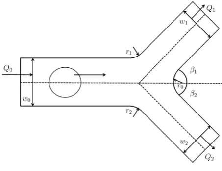
[image:7.595.311.538.551.725.2]

The geometry of a bifurcated blood vessel is shown in Figure 2, where w0 is the diameter of the mother vessel;

1

w and w2 are the diameters of the daughter vessels on the top and the bottom, respectively; β₁ and β₂ are the respective branching angles of the daughter vessels; the branching fillet radii r0, r1 and r2 are given as 3μm to make the vessel branching transition smooth; Q0, Q1 and Q2 represent the flow rate of each vessel. A RBC is placed near the inlet of the vessel. The radius of the RBC is also given as 2.66 μm. The incoming velocity of the mother vessel is set to be a constant as 0.1 cm/s. The branching angles β1 and β2 are set to be equal and constant, β1=β2=π 4. In this study, we set the diameter of the mother branch to be w0=8 μm, and consider two sets of diameter ratios, rd =w w1 2, to be 1 and 1.44. When the diameter ratio is 1, it is considered as symmetric bifurcation; when it is not 1, then it is considered as asymmetric.

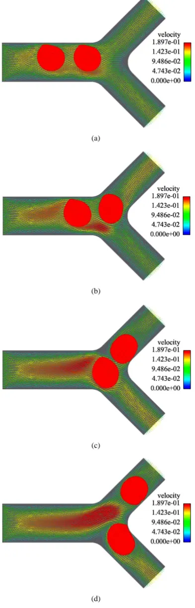
Figures 3 and 4 represent the blood cell behaviors when encountering bifurcation in symmetric and asymmetric vessels with different original positions and ratios of flow rate of each daughter vessel. Based on Figure 3 we can notice that although the daughter branches are symmetric in the geometry, due to the asymmetric boundary conditions where the ratio of the flow rates for the two daughter branches is Q Q1 2=3, the blood cell tends to move to the daughter branch with a higher mass flow rate. When the daughter branches are asymmetric in geometry but with the same mass flow rate Q Q1 2 =1, as shown in Figure 4, the blood cell moves to the one with a smaller cross section area, which is due to the higher average velocity in that daughter branch.

A multi-blood cell case is also simulated and the result is shown in Figure 5. The cell-to-cell interaction can be

(8)

(a)

(b)

(c)

(d)

Figure 3. A RBC owing in a symmetric bifurcated vessel with Q Q1 2=3. (a) t = 0.008 s; (b) t = 0.012 s;

(c) t =0.016 s; (d) t = 0.020 s.

(a)

(b)

(c)

(d)

Figure 4. A RBC flowing in an asymmetric bifurcation vessel with Q Q1 2=1. (a) t = 0.00 s; (b)

[image:8.595.65.517.74.691.2] [image:8.595.70.280.91.697.2]

(9)

(a)

(b)

(c)

[image:9.595.75.272.90.703.2]

(d)

Figure 5. Two RBCs in a symmetric bifurcation. (a)

t = 0.004 s; (b) t = 0.008 s; (c) t =0.012 s; (d) t = 0.018 s.

thought as two parts: 1) one cell changes the deformation and motion of the other cells by directly contacting each other; 2) one cell affects the other cells indirectly by changing the surrounding fluid field. For this case, in- stead of specifying the flow rate ratio between the daughter vessels, a constant inlet flow rate is given. Therefore, by simulating two RBCs laying in a line profile going through the symmetric bifurcation together, we are able to see this indirect cell-to-cell interaction. From these simulation results, the IFEM is proved to be suitable to simulate the red blood cell motion and deformation in microvessel bifurcation.

6.2. Deployment of Angioplasty Stents

For individuals with an occlusive vascular disease, blood flowing to an organ or to a distal body part is impaired by narrowed arteries with fatty deposits or calcium accumu- lations. Angioplasty was introduced by Dr. Andreas Gru- entzig in the mid to late 1970’s and is widely used today. The area of arterial blockage is dilated with the help of a catheter that has an inflatable small balloon at its tip. Then, the plaque is squeezed along the artery wall. A decade later, stenting was introduced by Dr. Julio Palmaz in 1988 to improve the angioplasty procedure. Like angioplasty, coronary stents physically open the channel of constricted arterial segments. During stenting, a catheter delivers a balloon and a surrounding stent to the location of the blockage area. The balloon deploys the stent, re- mains inflated for 30 seconds and then is deflated. At the end of the process, the expanded stent is embedded into the wall of the diseased artery and holds it open.

Here, we mainly focus on the deployment process of balloon-expanding stents. Balloon expandable stents are typically made of stainless steel tubing mounted over an angioplasty balloon and then plastically deformed to their final diameter by high pressure balloon inflation.

(10)

an increased intimal growth due to more profound and deep vascular injury. Shear stress, exerted on both the vascular wall and on the blood constituents, is considered to play an important role in restenosis. Therefore, besides biocompatibility issues, the design of both the stent and delivery mechanisms should receive the necessary atten-tion during the development process of the future gener-ation of stents.

In our previous work [27], we built a computer model and simulated a balloon expandable stent interacting with its surrounding fluid using the immersed finite element method. The initial configuration of the balloon and stent are designed and discretized using SolidWorks [43] and imported into our IFEM code. With the previously derived computational algorithm, the displacement and stress distribution of the stent and the velocity profile of the fluid domain can be obtained and analyzed. A balloon is designed with deflated tips at its two ends in its initial undeformed configuration, as shown in Figure 6(a). A catheter is located inside the balloon to apply appropriate pressure to inflate the balloon. The balloon has a length of 15 mm, an outer diameter of 1.54 mm, and a thickness of 0.04 mm. Both ends of the balloon are fixed in all directions as shown in Figure 6(b).

The balloons used for stenting are made of very stiff polyamide (nylon) material [44,45]. The balloon is mod- eled as hyperelastic material with Mooney-Rivlin description in the simulation. The parameters and material properties used for the balloon are summarized in Table 1.

A stent is a cylindrical and symmetrical assembly of inter-connected diamond-shaped members. In this particular model, we use the Medtronic AVE Modular stents S7 (Medtronic AVE, Inc., Santa Rosa, CA, USA), Figure 7(a). Although this stent is no longer been widely used, it is still a good representation of a typical geometrical shape of a stent, the model can be simply modified to other expandable devices. The stent, made of wires that form a diamond shape as shown on Figure 7(b), has an outer diameter of 1.64 mm. The stent is made of 16 identical structural members with a total length of 8 mm before its expansion. The cross-section of the wire has a width of 0.08 mm. The structural members are connected peak-to- peak at their tips. Balloon-expandable stents are made from materials that can be plastically deformed through the inflation of a balloon. An ideal stent should have low yield stress (to make it deformable at manageable balloon pressures), high elastic modulus (for minimal recoil), and high strength through expansion. The most widely used material for this type of stents is stainless steel, typically 316 L, a particular corrosion-resistant material. For stents the fatigue resistance is of high impor- tance. Therefore, the microstructure requires very small

Table 1. Parameters and material properties used for the balloon.

5929 nodes Length = 15 mm Density= 3000 kg/m3

17,846 elements Diameter = 1.54 mm Shear modulus = 300 Pa

Thickness = 0.04 mm Bulk modulus = 1500 Pa

(a)

(b)

Figure 6. Balloon geometry setup. (a) Initial balloon geometry before inflation; (b) Fixed boundaries applied at the two ends of the balloon.

(a) (b)

Figure 7. Design of a Medtronic AVE Modular stents S7. grain sizes. The typical average grain sizes of approx- imately 25 μm exist in stainless steel stents and 8 to 9 grains over the strut wall thickness are desired [46]. We assume a clean homogeneous material with a uniformly fine grain size and a near 100% density. Stainless-steel alloys are usually preferred to design stents because they have been proven to be biocompatible for long-term im- plants in the human body and easily deformable in fully annealed condition. The stent is discretized using 9.979 nodes and 16.888 elements. A summary of the properties and parameters used for the stent is listed in Table 2.

Finally, the stent is mounted around the balloon as shown in Figure 8. The stent is placed at the center of the balloon. At this point, several assumptions must be made: 1) the force applied on the balloon is transferred directly to the stent; 2) there is no fluid between the balloon and the stent; and 3) the contact surface between the balloon and the stent is frictionless.

(11)

[image:11.595.309.538.101.242.2]

Table 2. Parameters and material properties used for the stent.

9979 nodes Length = 8 mm Density = 4000 kg/m3

16,888 elements Diameter = 1.64 mm Shear modulus = 300 Pa

Thickness = 0.08 mm Bulk modulus = 1500 Pa

Figure 8. Initial configuration of catheter, ballon, and stent. 4.5 mm. Our computational model assumes that the fluid is everywhere in the domain. Although the balloon is not inflated with the same fluid as the surrounding blood, a liquid (with color) that has similar properties as the blood is normally inserted into the balloon for easier visualiza- tion in surgeries. Therefore, it is a reasonable assumption to have homogeneous fluid in the entire computational domain. Blood is an incompressible fluid consisting of a suspension of deformable particles (blood cells, platelets, etc.) in a Newtonian liquid (plasma). Except within the microcirculation, blood can be considered homogeneous with constant density and viscosity. The parameters and properties used for the fluid domain to perform the simulation can be found in Table 3.

The crimped stent is deformed by a radial force from the balloon. Experiments performed by Dumoulin and Cochelin [47], and Moore and Berry [48] showed that, except at the tips, the structure is almost uniformly dilated and finally expanded. Thus, it seems justifiable to model expansion by considering a long structure under uniform radial internal pressure. This pressure difference is applied from the centerline towards the outer diameter of the balloon and the artery wall, as shown on Figure 9. The applied inflation pressure is dependent on the struts of the wires and the specific material used. The total inflation pressure for the balloon is equal to the sum of the pressure required to deform the balloon material and to deploy the stent. During the entire simulation the inflation pressure is constant and equals to 100 g/cm2.

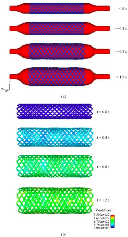
Our primary goal is to study the deformation of the stent during its deployment. Figure 10(a) shows the deployment of the stent during balloon expansion at different time steps. The pressure applied onto the fluid inflates the balloon and the balloon provides a force onto the stent, which enables the stent to expand radially outward until it contacts the inner surface of the artery wall.

During deployment, the diameter of the stent increases from 1.64 mm to 2.82 mm. As expected, the stent deforms uniformly in its radial direction, expanding by 1.7 times its initial diameter for our given material. Figure 11(a) shows that the expansion of the stent in its radial direction follows a linear variation.

Figures 10(a) demonstrates how the diamond shape of

Table 3. Parameters and properties used for the fluid domain.

4348 nodes Length = 16 mm Density = 1000 kg/m3

20,568 elements Diameter = 4.5 mm Viscosity = 0.01 N∙s/m2

Figure 9. The initial conditions applied to the fluid domain: constant pressure difference (P2− P1) is applied from the ca-

theter to the fluid boundaries.

(a)

(b)

[image:11.595.59.285.102.192.2] [image:11.595.312.536.288.700.2]

(12)

(a)

[image:12.595.311.537.85.350.2]

(b)

[image:12.595.89.258.86.340.2]

Figure 11. Stent diameter and maximum von Mises stress vs. time during stent deployment. (a) Stent diameter variation during the deployment; (b) Maximum Von Mises stress variation during the deployment.

the stent deforms during the deployment. Compared to experiments and observations of deployment of a real stent, our three-dimensional computational model gives a realistic representation of stent expansion during balloon inflation.

[image:12.595.309.535.378.631.2]

The strength and the long term in-vivo performance of the stent can be determined from the stress distributions with the goal of minimizing vascular injury. The Von Mises stress distribution along the stent is reported at different time steps in Figure 10(b). The stress distribution is uniform longitudinally along the stent and varies during deployment. The highest stress values appear at the final stage of expansion, and the peak Von Misses stress follows a linear variation during the entire simulation as shown on these values are critical for recoil and failure analysis. It can be concluded that the stress distribution is a function of applied pressure, balloon and stent material properties, fluid properties, and stent geometry. Figure 12 shows the radial fluid velocity profile during the deployment of the stent. This profile represents better how the applied uniform pressure acts on the balloon in the radial direction. Figure 13 shows the magnitude and profile of the velocity in the transverse plane. Both figures demonstrate a uniform velocity distribution in the direction of expansion, illustrating how well our model simulates the expansion mechanism through applied pressure difference.

Figure 12. Radial fluid velocity profile at different time steps.

Figure 13. Velocity profile in the longitudinal direction during expansion at different time steps.

6.3. Human Vocal Folds Vibration during Phonation

(13)

[image:13.595.308.538.85.188.2]

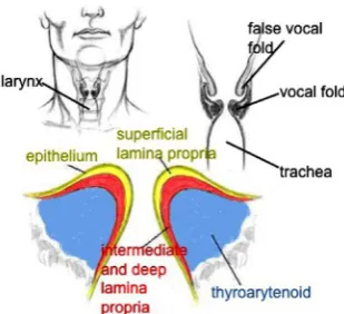
Figure 14. Human vocal folds.

human vocal folds are roughly 10 - 15 mm in length and 3 - 5 mm thick. The human vocal folds are laminated structures composed of five different layers: the epithe- lium, the superficial layer (SLP), the intermediate layer (ILP), the deep layer and thyroarytenoid muscle, shown in Figure 14.

An accurate numerical simulation of the vocal folds vibration can help us obtain a better understanding of the dynamics of the voice production in human beings. Due to the complicated nature of this problem, the numerical model has to fulfill the following requirements. First, the numerical model has to represent completely a coupled fluid-structure interaction system. Second, the numerical model should perform well when there exists large density ratio between the fluid and structure because the density of the vocal fold muscle is close to water and the density ratio between the vocal fold muscle and the airflow is about 1000. Third, the motion and deformation of the structure have to be predicted accurately with complicated geometry and material descriptions because the vocal folds have complex shape and layer-structures and are viscoelastic materials. The mIFEM is a perfect numerical method to perform the simulation of this com-plex problem.

The geometry of the self-oscillated vocal folds model is shown in Figure 15. Since sound is generated by the compression of air, the working fluid is taken as compressible air governed by the ideal gas law at room tem- perature. The density of the fluid is

3 3

1.3 10 g/cm

f

ρ ₌ _× −

and the viscosity of the fluid is

4 1.8 10 g/cm s

µ₌ _× − _⋅

.

The vocal fold muscle is considered as isotropic viscoelastic material. The vocal fold is assumed to have layered structure, outside cover layer (red) and inside body layer (green). The cover layer is much softer than the body layer. For the cover layer the Young’s modulus is E=10 kPa, whereas E=40 kPa for the body layer. The densities of both cover and body layer are assumed

to be the same as 3

1.0g/cm

s

ρ = . The Poisson ratio is

0.3

ν= . Two vocal folds have the exact same geometry

Figure 15. 2-D two-layer self-oscillated vocal folds model. and material description, sit in the fluid channel symmetric about the central line. A constant total pressure boundary condition of Pin =1 kPa is applied at the channel inlet and the outflow boundary is given at the channel exit. No-slip and no-penetration boundary conditions are applied on the channel walls and on the vocal fold surfaces.

A snapshot of the fluid velocity field at two typical instances during a steady vibration cycle are shown in Figure 16. One can see that the fluid field is not symmetric about the central line during the vibration. The glottal jet tends to attach to one side of the vocal folds randomly, which is the so-called the “Coanda effect” [49,50].

The asymmetrical airflow causes an asymmetrical pressure distribution in regions near the vocal folds and change in the vibration pattern. The minimum distance between the vocal fold surface and the central line is measured to represent the half glottis width

( )

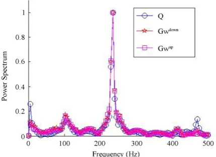
Gw , shown in Figure 17, where Gwup and Gwdown represent

the opening width for the up and down vocal folds, respectively. This figure shows that the simulation captures the vocal folds to have a repeated opening and closing process. When the glottis width is zero or near-zero, then the vocal folds are closed, there is no air flowing through. The pressure starts to build up in the upstream of the vocal channel. As the pressure increases, it starts to push the vocal folds to open and eventually reaches a maximum glottis width, the high pressure is released. The vocal folds then return back to its closed position, and the whole process restarts. The glottis width for the up and down vocal folds do not equal each other over cycles, indicating that the vocal folds motion is asymmetric although the vibrational frequency is found to be the same. The vibrational magnitude is slightly off from each other. To find out the vibration frequency, FFT is performed on the up and down glottis widths and the volume flow rate, Q. The power spectra are plotted in Figure 18 where the frequency for these three variables are the same and found to be 234 Hz, which is in the expected range of a female vocal fold vibrational frequency.

7. CONCLUSION

[image:13.595.94.249.86.227.2]

(14)

[image:14.595.59.289.86.264.2] [image:14.595.65.283.306.462.2]

Figure 16. Fluid velocity field at two typical instances during steady vibration.

Figure 17. Half glottis width of top and bottom vocal folds.

Figure 18. Spectrum plot of flow rate and half glottis width of the top and bottom vocal folds.

been developed over the past decade. The IFEM method is a numerical scheme that adopts the non-boundary-fitted mesh approach and fully couples the fluid-structure interaction by interpolation of the interacting domains.

The fluid and solid domains are solved independently using finite element method and coupled with each other within one time step through fluid-structure interaction force. The original IFEM algorithm is considered as ex-plicitly coupling for the fluid and solid, which can lead to instability issue when time step is not sufficiently small. The semi-implicit IFEM algorithm tackles this problem by modifying the FSI force and adopting the concept of the indicator function. It extends the stability range of the numerical scheme and allows us to consider the fluid- structure interaction problems when the fluid and solid properties are very different from each other, for example high density ratio between the solid and fluid, and the solid with relatively large stiffness. For high Reynolds number flows,, the modified IFEM algorithm performs better due to its accurate description of the solid motion and deformation through capturing the dynamics of the solid motion. Three biomedical applications are studied using these IFEM algorithms to simulate soft tissues in-teracting with fluid where the fluid can be either blood or air.

ACKNOWLEDGEMENTS

This work is partially funded by NIH (R01-DC005642-07).

REFERENCES

[1] Peskin, C. (1977) Numerical analysis of blood flow in the heart. Journal of Computational Physics, 25, 220-252. http://dx.doi.org/10.1016/0021-9991(77)90100-0

[2] McCracken, M. and Peskin, C. (1980) A vortex method for blood flow through heart valves. Journal of

Computa-tional Physics, 35, 183-205.

http://dx.doi.org/10.1016/0021-9991(80)90085-6

[3] McQueen, D. and Peskin, C. (1983) Computer-assisted design of pivoting-disc prosthetic mitral valves. Journal

of Computational Physics, 86, 126-135.

[4] Peskin, C. and McQueen, D. (1989) A three-dimensional computational method for blood flow in the heart. I. Im-mersed elastic fibers in a viscous incompressible fluid.

Journal of Computational Physics, 81, 372-405.

http://dx.doi.org/10.1016/0021-9991(89)90213-1

[5] Peskin, C. and McQueen, D. (1992) Cardiac fluid dy-namics. Critical Reviews in Biomedical Engineering,

SIAM Journal on Scientific and Statistical Computing, 20,

451-459.

[6] Peskin, C. and McQueen, D. (1994) Mechanical equili-brium determines the fractal fiber architecture of aortic heart valve leaflets. American Journal of Physiology, 266, H319-H328.

[7] Peskin, C. and McQueen, D. (1996) Case studies in ma-thematical modeling-ecology, physiology, and cell biol-ogy. Prentice-Hall, Upper Saddle River.

[image:14.595.65.280.493.649.2]

(15)

coeffi-cients and singular sources. SIAM Journal on Numerical

Analysis, 31, 1091-1044.

http://dx.doi.org/10.1137/0731054

[9] LeVeque, R.J. and Li, Z. (1997) Immersed interface me-thods for stokes flow with elastic boundries or surface tension. SIAM Journal on Scientific Computing, 18, 709- 735. http://dx.doi.org/10.1137/S1064827595282532

[10] Fogelson, A. and Keener, J. (2000) Immersed interface method for Neumann and related problems in two and three dimensions. SIAM Journal on Scientific Computing, 22, 1630-1654.

http://dx.doi.org/10.1137/S1064827597327541

[11] Lee, L. and LeVeque, R. (2003) An immersed interface method for incompressible Navier-Stokes equations, SIAM

Journal on Scientific Computing, 25, 832-856.

http://dx.doi.org/10.1137/S1064827502414060

[12] Li, Z. and Lai, M. (2001) The immersed interface method for the Navier-Stokes equations with singular forces. Jour-

nal of Computational Physics, 171, 822-842.

http://dx.doi.org/10.1006/jcph.2001.6813

[13] Wiegmann, A. and Bube, K.P. (1998) The immersed interface method for nonlinear differential equations with discontinuous coefficients and singular sources. SIAM

Journal on Numerical Analysis, 35, 177-200.

http://dx.doi.org/10.1137/S003614299529378X

[14] Wiegmann, A. and Bube, K.P. (2000) The explicit-jump immersed interface method: Finite difference methods for PDEs with piecewise smooth solutions. SIAM Journal on

Numerical Analysis, 37, 827-862.

http://dx.doi.org/10.1137/S0036142997328664

[15] Wang, X. and Liu, W. (2004) Extended immersed boun-dary method using FEM and RKPM. Computer Methods

in Applied Mechanics and Engineering, 193, 1305-1321.

http://dx.doi.org/10.1016/j.cma.2003.12.024

[16] Boffi, D. and Gastaldi, L. (2003) A finite element ap-proach for the immersed boundary method. Computers

and Structures, 81, 491-501.

http://dx.doi.org/10.1016/S0045-7949(02)00404-2

[17] Boffi, D., Gastaldi, L. and Heltai, L. (2007) On the CFL condition for the finite element immersed boundary me-thod. Computers and Structures, 85, 775-783.

http://dx.doi.org/10.1016/j.compstruc.2007.01.009

[18] Wang, S.X., Zhang, L.T. and Liu, W.K. (2009) Finite element formulations for immersed methods: Explicit and implicit approaches. Journal of Computational Physics, 228, 2535-2551.

http://dx.doi.org/10.1016/j.jcp.2008.12.012

[19] Zhang, L., Gerstenberger, A., Wang, X. and Liu, W. (2004) Immersed finite element method. Computer Methods in

Applied Mechanics and Engineering, 193, 2051-2067.

[20] Zhang, L. and Gay, M. (2007) Immersed finite element method for fluid-structure interactions. Journal of Fluids

and Structures, 23, 839-857.

http://dx.doi.org/10.1016/j.jfluidstructs.2007.01.001

[21] Zhang, L.T. and Gay, M. (2008) Imposing rigidity con-straints on immersed objects in unsteady fluid flows.

Computational Mechanics, 42, 357-370.

http://dx.doi.org/10.1007/s00466-008-0244-8

[22] Wang, X. and Zhang, L.T. (2010) Interpolation functions in the immersed boundary and finite element methods.

[23] Liu, W., Liu, Y., Farrell, D., Zhang, L., Wang, S., Fukui, Y., Patankar, N., Zhang, Y., Bajaj, C., Lee, J., Hong, J., Chen, X. and Hsu, H. (2006) Immersed finite element method and its applications to biological systems. Com-

puter Methods in Applied Mechanics and Engineering,

195, 1722-1749.

[24] Liu, W., Liu, Y., Zhang, L., Wang, X., Gerstenberger, A. and Farrell, D. (2004) Immersed finite element method and applications to biological systems. Finite Element Methods: 1970’s and Beyond. International Center for Numerical Methods and Engineering.

[25] Liu, Y. and Liu, W. (2006) Rheology of red blood cell aggregation in capillary by computer simulation. Journal

of Computational Physics, 220, 139-154.

http://dx.doi.org/10.1016/j.jcp.2006.05.010

[26] Liu, Y., Zhang, L., Wang, X. and Liu, W. (2004) Coupl-ing of Navier-Stokes equations with protein molecular dynamics and its application to hemodynamics.

Interna-tional Journal for Numerical Methods in Fluids, 46,

1237-1252. http://dx.doi.org/10.1002/fld.798

[27] Gay, M., Zhang, L. and Liu, W. (2006) Stent modeling using immersed finite element method. Computer Me-

thods in Applied Mechanics and Engineering, 195, 4358-

4370. http://dx.doi.org/10.1016/j.cma.2005.09.012

[28] Zhang, L.T. (2008) Shear stress and shear-induced par-ticle residence in stenosed blood vessels, International

Journal of Multiscale Computational Engineering, 6,

141-152.

http://dx.doi.org/10.1615/IntJMultCompEng.v6.i2.30

[29] Zhang, L.T. and Gay, M. (2008) Characterizing left atrial appendage functions in sinus rhythm and atrial fibrillation using computational models. Journal of Biomechanics, 41, 2515-2523.

http://dx.doi.org/10.1016/j.jbiomech.2008.05.012

[30] Gay, M. and Zhang, L.T. (2009) Numerical studies of healthy, stenosed, and stented coronary arteries.

Interna-tional Journal of Numerical Methods in Fluids, 61, 453-

472. http://dx.doi.org/10.1002/fld.1966

[31] M. Gay, and L. T. Zhang, (2009) Numerical studies on fluid-structure interactions of stent deployment and stented arteries. Engineering with Computers, 25, 61-72. http://dx.doi.org/10.1007/s00366-008-0105-2

[32] Tezduyar, T. (1992) Stabilized finite element formula-tions for incompressible-flow computaformula-tions. Advanced Ap-

plication Mechanics, 28, 1-44.

[33] Tezduyar, T. (2001) Finite element methods for flow problems with moving boundaries and interfaces. Archives of

Computational Methods in Engineering, 8, 83-130.

http://dx.doi.org/10.1007/BF02897870

(16)

accommodating equal-order interpolations. Computer Me-

thods in Applied Mechanics and Engineering, 59, 85-99.

http://dx.doi.org/10.1016/0045-7825(86)90025-3

[35] Wang, X., Wang, C. and Zhang, L.T. (2011) Semi-implicit formulation of the immersed finite element method.

http://dx.doi.org/10.1007/s00466-011-0652-z

[36] Wang, X. and Zhang, L.T. (2013) Modified immersed finite element method for solid-dominated fully-coupled fluid-structure interactions. Computer Methods in Com-

puter Methods in Applied Mechanics and Engineering,

267, 150-169.

[37] Peskin, C. (2002) The immersed boundary method. Acta

Numerica, 11, 479-517.

http://dx.doi.org/10.1017/S0962492902000077

[38] Torres, D. and Brackbill, J. (2000) The point-set method: front-tracking without connectivity. Journal of

Computa-tional Physics, 165, 620-644.

http://dx.doi.org/10.1006/jcph.2000.6635

[39] Colombo, A., Hall, P., Nakamura, S., Almagor, Y., Ma- iello, L., Martini, G., Gaglione, A., Goldberg, S. and To- bis, J. (1995) Intracoronary stenting without anticoagulation accomplished with intravascular ultrasound guidance.

Circulation, 91, 1676-1688.

http://dx.doi.org/10.1161/01.CIR.91.6.1676

[40] Goldberg, S., Colombo, A., Nakamura, S., Almagor, Y., Maiello, L. and Tobis, J. (1994) Benefit of intracoronary ultrasound in the deployment of Palmaz-Schatz stents.

Journal of the American College of Cardiology, 24, 996-

1003. http://dx.doi.org/10.1016/0735-1097(94)90861-3

[41] Segers, P., Kostopoulos, K., Scheerder, I.D. and Ver-donck, P. (1998) Biomechanical aspects of intracoronary stents. In: Verdonck, P., Ed., Intra and Extracorporeal

Cardiovascular Fluid Dynamics, Vol. 1, General Princi-

ples in Application, WIT Press, Ashurst, 203-232.

[42] Russo, R., Schatz, R., Sklar, M., Johnson, A., Tobis, J. and Teirstein, P. (1995) Ultrasound guided coronary stent placement without prolonged systemic anticoagulation.

Journal of the American College of Cardiology, 25, 50A.

http://dx.doi.org/10.1016/0735-1097(95)91662-H

[43] SolidWorks (2004) Sp03.1. SolidWorks Corporation, Concord.

[44] Serruys, P. and Rensing, B. (2002) Handbook of coronary stents. 4th Edition, Martin Dunitz, London.

[45] Saab, M. (1999) Applications of high-pressure balloons in the medical device industry. Advanced Polymers, Inc. Salem.

[46] Murphy, B., Savage, P., McHugh, P. and Quinn, D. (2003) The stress-strain behavior of coronary stent struts is size dependent. Annals of Biomedical Engineering, 31, 686- 691. http://dx.doi.org/10.1114/1.1569268

[47] Dumoulin, C. and Cochelin, B. (2000) Mechanical beha-vior modeling of balloon-expandable stents. Journal of

Biomechanics, 33, 1461-1470.

http://dx.doi.org/10.1016/S0021-9290(00)00098-1 [48] Moore Jr., J.E. and Berry, J. (2002) Fluid and solid

me-chanical implications of vascular stenting. Annals of

Biomedical Engineering, 30, 498-508.

http://dx.doi.org/10.1114/1.1458594

[49] Tao, C., Zhang, Y., Hottinger, D.G. and Jiang, J.J. (2007) Asymmetric airflow and vibration induced by the Coanda effect in a symmetric model of the vocal folds. Journal of

the Acoustical Society of America, 122, 2270-2278.

http://dx.doi.org/10.1121/1.2773960

[50] Drechsel, J.S. and Thomson, S.L. (2008) Influence of supraglottal structures on the glottal jet exiting a two- layer synthetic, self-oscillating vocal fold model. Journal

of the Acoustical Society of America, 123, 4434-4445.