Modeling the evolution of Gini coefficient for personal incomes in the USA between 1947 and 2005

Munich Personal RePEc Archive

Modeling the evolution of Gini coefficient

for personal incomes in the USA between

1947 and 2005

Kitov, Ivan

IDG RAS

April 2007

Online at

https://mpra.ub.uni-muenchen.de/2798/

Modeling the evolution of Gini coefficient for personal incomes in the USA between 1947 and 2005

Ivan O. Kitov

Introduction

The presence of economic inequality in any modern society is a trivial fact. There are

numerous economic theories of income distribution explaining this observation. Neal and

Derek (2000) provide a comprehensive overview of the state-of-art in this filed. In spite

of the efforts associated with the development of a consistent model of income

distribution there are numerous problems yet to resolve. Furthermore, the modern

economic theories do not meet some fundamental requirements applied to any scientific

theory - a concise description of accurately measured variables and prediction of their

evolution beyond the period of currently available measurements.

The most popular aggregate measure of economic inequality is the Gini

coefficient. This coefficient is characterized by a number of advantages such as relative

simplicity, anonymity, scale independence, and population independence. On the other

hand, the Gini coefficient belongs to the group of operational measures: its evolution in

time is not theoretically linked to macroeconomic variables and the differences observed

between countries are not well explained. These caveats make the Gini coefficient more

useful in political and social applications not in economics as a potentially hard science.

As a rule, the Gini coefficient is estimated from household surveys and inequality

is reported at family and household level of aggregation. Such an aggregation involves

social and demographic processes biasing pure economic mechanisms affecting the

inequality. Theoretically, the indivisible level for an inequality study is personal income,

which is assumed to be sensitive only to macroeconomic variables. There are just few

studies devoted to the Gini coefficient for personal income distribution (PID), however.

For example, the US Census Bureau (2006) has been publishing individual Gini

coefficients estimated from Current Population Surveys (CPS) since 1994.

Kitov (2005a, 2005b, 2005c, 2006a) has developed a model describing observed

personal income distribution in the USA and its evolution through time. This model is

based on the prediction of each and every individual income for the population 15 years

work experience, the evolution of PID in narrow age groups, and the number of people

and age dependence in the income zone described by the Pareto distribution. The model

also provides predictions for these variables beyond the years where corresponding data

are available. Having a complete and precise description of the US PID evolution one can

compute relevant Gini coefficients. This makes the Gini coefficient only of secondary

importance because its evolution is completely described by the evolution of the PID,

which is an exactly modeled function.

The purpose of this study is to accurately estimate the Gini coefficients associated

with the personal income distributions provided by the US Census Bureau and to model

the evolution of these coefficients between 1947 and 2005, i.e. during the period of

continuous PID measurements. For this purpose, an extended analysis of the PIDs has

been carried out and the discrepancy between the observed and predicted Gini

coefficients is interpreted in the framework of the changing accuracy and methodology,

including income definitions, of the CPS during the studied period.

The reminder of the paper is organized as follows. Section 1 introduces the model

for the evolution of individual incomes in the USA. Section 2 describes the data on

personal income distribution and presents some estimates of Gini coefficients according

to various data sets and definitions of income. Section 3 compares the evolution of the

observed Gini coefficients with those predicted by the model. Section 4 concludes.

1. The model for the evolution of income distribution

The principal assumption of the microeconomic model is that every person above

fourteen years of age has a capability to work or earn money using some means, which

can be a job, bank interest, stocks, interfamily transfers, etc. An almost complete list of

the means is available in the US Census Bureau technical documentation (2002) as the

sources of income are included in the survey list. Some principal sources of income are

not included, however, what results in the observed discrepancy between aggregate

(gross) personal income, GPI, and GDI.

Here we introduce the model described by Kitov (2005a). The rate of income, i.e.

the overall income a person earns per unit time, is proportional to her/his capability to

only source of any goods and services denominated in monetary units.) The person is not

isolated from the surrounding world and the work (money) s/he produces dissipates

(conventional economic term for the process would be depreciation, but physical terms

are more appropriate in this case) through interaction with the outside world, decreasing

the final income rate. The counteraction of external agents, which might be people or any

other externalities, determines the price of the goods and services a person creates. The

price depends not on some absolute measure of quality of the goods but on the aggregate

opinion of the surrounding people on relative merits (expressed in monetary units) of the

producers not goods. For example, the magic of famous brands provides a significant

increase in incomes for their owners without proportional superiority in quality because

people appreciate the creators not goods. As a whole, an equilibrium system of prices

arises from the aggregate opinions on relative merits of each and every person not from

the physical quantities and qualities of goods and services. The personal incomes are

ranked in some fixed hierarchy and, when expressed in monetary units, the hierarchy is

transformed in the dynamic system of prices. Since the hierarchy of incomes is fixed, the

amounts and qualities of goods can only reorder individuals not change the final

aggregate price of everything produced – GDP.

Analogously to many cases observed in natural sciences, the rate of dissipation is

proportional to the attained income (per unit time) level and inversely proportional to the

size of the means used to earn the money, Λ. Bulk heating of a body accompanied by

cooling through its surface is the case. For a uniform distribution of heating sources, the

energy released in the body is proportional to its volume or cube of characteristic linear

size and the energy lost through its surface is proportional to the square of the linear size.

In relative terms, the energy balance or the ratio of cooling and heating is inversely

proportional to the linear size. As a result, a larger body undergoes a faster heating

because loses relatively less energy and also reaches a higher equilibrium temperature.

Therefore one can write an ordinary differential equation for the changing rate of income

earned by a person in the following form:

where M(t) is the rate of money income denominated in dollars per year [$/y], t is the

work experience expressed in years [y], σ(t) is the capability to earn money [$/y2]; and α

is the dissipation coefficient expressed in units [$/(y2)]. The size of the earning means, Λ,,,,

is also expressed in [$/y]. The general solution of equation (1), if σ(t) and Λ(t) are

considered to be constant (because these two variables evolve very slowly with time), is

as follows:

M(t)=(σ/α)Λ(1-exp(-αt/Λ)) (2)

In the modeling, we integrate (1) numerically in order to include the effects of the

changing σ(t) and Λ(t). Equations (2) through (4) are derived and discussed in detail

below to demonstrate some principal features of the model. These equations represent the

solutions of (1) in the case where the observed change in σ(t) and Λ(t) in all the terms is

neglected.

One can introduce the concept of a modified capability to earn money as a

dimensionless variable Σ(t)=σ(t)/α. . . . The absolute value of the modified capability, Σ(t),

and the size of earning means evolves with time as the square root of real GDP per

capita:

Σ(t)= Σ(t0)sqrt(GDP(t)/GDP(t0))

and

Λ(t)= Λ(t0)sqrt(GDP(t)/GDP(t0)),

where GDP(t0)and GDP(t)are the per capita values at the start point of the modeling, t0,

and at time t, respectively. Then the capacity of a “theoretical” person to earn money,

defined as Σ(t)Λ(t), evolves with time as real GDP per capita. Effectively, equation (2)

states that the evolution in time of a personal income rate depends only on the personal

capability to earn money, the size of the means used to earn money, and the economic

growth.

The modified capability to earn money,Σ(t), and the size of earning means, Λ(t),

respectively. One can now introduce relative and dimensionless values of the defining

variables in the following way:S(t)=Σ(t)/ΣBminB(t)and L(t)=Λ(t)/ΛBminB(t).

A fundamental assumption is made that the possible relative values of S(t0) and

L(t0) can be represented as a sequence of integer numbers from 2 to 30, i.e. only 29

different integer values of the relative S(t0) and L(t0) are available: SB1B=2,…, SB29B=30;

LB2B=2,…, LB29B=30. This discrete range results from the calibration process described by

Kitov (2005a). The largest possible relative value of SBmaxB=SB29B=30=LBmaxB=LB29B is only 15

(=30/2) times larger than the smallest possible S=SB1B and L=LB1B (in the model, the

minimum values ΛBminB and ΣBminB are chosen to be two times smaller than the smallest

observed valuesofΛB1B and ΣB1B). Because the absolute values of variables Λi, Σi, ΛBminB, and

ΣBminBevolve with time according to the same law, the relative and dimensionless variables

LBiB(t) and SBiB(t), i=1,…,29, do not change with time retaining the discrete distribution of

relative values. This means that the distribution of the relative capability to earn money

and the size of earning means is fixed as a whole over calendar years and also over ages.

This assumption on the rigid character of the hierarchy of incomes is supported by

observations, as presented by Kitov (2005a, 2005b) for the period between 1994 and

2002. This study extends the set of observations to the period between 1947 and 2005.

In equation (2), one can substitute the product of the relative values S and L and

the time dependent minimum values ΛBminB andΣBminB for Σ(t) and Λ(t). We also normalize

the equation to the maximum values SBmaxB and LBmaxB. The normalized equation for the rate

of income, MBijB(t), for aperson with the capability, SBiBand the size of earning means,LBjBis

as follows:

MBijB(t)/(SBmaxBLBmaxB ) = (ΣBminBΛBminB)(SBiB/SBmaxB)(LBjB/LBmaxB)(1 - exp(-(α/ΛB minB LBmaxB)t/(LBjB/LBmaxB)))(3)

or

M'BijB(t) =ΣBminB(t)ΛBminB(t)S'BiBL'BjB{1 - exp[-(1/ΛBminB)(α't/L'BjB)]} (3’)

where M'BijB(t)=MBijB(t)/(SBmaxBLBmaxB); S'BiB=(SBiB/SBmaxB); L'BjB=(LBjB/LBmaxB); α'=α/LBmaxB, SBmaxB=30, and

LBmaxB=30. Below we omit the prime indices. The term ΣBminB(t)ΛBminB(t) corresponds to the

experience, t (t0=0), and is different for different years of birth. This term might be

considered as a coefficient defined for every single year of work experience because this

is a predefined external variable. Thus, one can always measure the personal income in

units ΣBminB(t0)ΛBminB(t0). Then equation (3') becomes a dimensionless one and the coefficient

changes from 1.0 as the real GDP per capita evolves relative to the start year.

Equation (3’) represents the rate of income for a person with the defining

parameters SBiB and LBjB at time t relative to the maximum possible personal income rate.

The maximum possible income rate is obtained by a person with SB29B=30/30=1 and

LB29B=30/30=1 at the same time t. The term 1/ΛBminB in the exponential term evolves

inversely proportional to the square root of real GDP per capita. This is the defining term

of the personal income evolution, which accounts for the differences between the start

years of work experience. The numerical value of the ratio α/ΛBminB is obtained by

calibration for the start year of the modeling. This calibration assumes that ΛBminB(t0)=1

(and ΣBminB(t0)=1 as well) at the start point of the modeling and only the dimensionless

factor α has to be empirically determined. In thiscase, absolute value of α depends on

start year.

As numerous observations show, the money earning capacity, SBiBLBjB, drops to zero

at some critical time, TBcrB, in a personal history (Kitov, 2005a), the solution of (1) is:

MBijB(t) =

MBijB(Tcr)exp(-α (t-Tcr)/ ΛBminB LBjB) =

= {ΣBminB(t)ΛBminB(t)SBiBLBjB(1-exp(-αTcr/ΛBminB LBjB))} exp(-α1(t-Tcr)/ ΛBminB LBjB) (4)

The first term is equal to the level of income rate attained by the person at time TBcrB, and

the second term represents an exponential decay of the income rate for work experience

above TBcrB. The exponent index α1 is different from α and varies with time. It was found

that the exponential decrease of income rate above Tcr results in the same relative (as

reduced to the maximum income for this calendar year) income rate level at the same

age. It means that the index can be obtained according to the following relationship:

where C is the constant relative level of income rate at age A. Thus, when current age

reaches A the maximum possible income rate Mij (for i=29and j=29) drops to C. Income

rates for other values of i and j are defined by (4). For the period between 1994 and 2002,

empirical estimates are as follows: C=0.72 and A=64 years. The observed exponential

roll-off for individual and the mean income beyond TBcrB corresponds to a zero-value work

applied to earn money in the model. People do not exercise any effort to produce income

starting from some predefined (but growing) point in time, TBcrB, and enjoy exponential

decay of their incomes. A physical analog of such decay is cooling of a body, for

example, the Earth. When all sources of internal heating (gravitational, rotational, and

radioactive decay) disappear, the Earth only will be loosing the internal heat through the

surface before reaching an equilibrium temperature with the outer space. This process of

cooling is also described by an exponential decay because the heat flux from the Earth is

proportional to the difference of the temperatures between the Earth’s surface and the

outer space.

The probability for a person to get an earning means of relative size LBjB is constant

over all 29 discrete values of the size. The same is valid for SBiB, i.e. all people of 15 years

of age and above are distributed evenly among the 29 groups for the capability to earn

money. Thus, the relative capacity for a person to earn money is distributed over the

working age population as the product of independently distributed SBiB and LBj - B SBiBLBj B=

{2×2/900, 2×3/900, …, 2×30/900, 3×2/900, …, 3×30/900, …, 30×30/900}. There are

only 841 (=29x29) values of the normalized capacity available between 4/900 and

900/900. Some of these cases seem to be degenerate (for example, 2x30=3x20=4x15=

…= 30x2), but actually all of them define different time histories according to (3’),

where LBjBis also present in the exponential term. In the model, no individual (in sense of

real people) future income trajectory is predefined, but it can only be chosen from the set

of the 841 predefined individual futures for each single year of birth.

It is not possible to quantitatively estimate the value of the dissipation factor,

α, , , , using some independent measurements. Instead, a standard calibration procedure is

applied. By definition, the maximum relative value of LBjB (LB29B) is equal to 1.0 at the start

can vary α in order to match predicted and observed PIDs, and the best-fit value of α is

used for further predictions. The range of α/ΛBminB from 0.09 to 0.04 approximately

corresponds to that obtained in the modeling of the US PIDs during the period between

1960 and 2002 (Kitov, 2005a). Actual initial value of α is found to be 0.086 for tB0B=1960.

The value of ΛBminB changes during this period from 1.0 to 1.49 according to the square

root of the real GDP per capita growth. The cumulative growth of the real GDP per

capita from 1960 to 2002 is 2.22 times.

Because the exponential term in (2) includes the size of earning means growing as

the root square of the real GDP per capita, longer and longer time is necessary for a

person with the maximumrelative values SB29Band LB29Bto reach the maximum income rate.

There is a critical level of income rate, however, which separates two income zones with

different properties. This level is called the Pareto threshold of income. Below this

threshold, in sub-critical income zone, PID is accurately predicted by the model for the

evolution of individual income. One can crudely approximate the PID by an exponent

with a small negative index, as shown later on in the paper. Above the Pareto threshold,

in supercritical income zone, PID is governed by a power (equivalent to the Pareto) law.

The presence of a high-income zone with the Pareto distribution allows any person

reaching the threshold to obtain any income in the distribution, with rapidly decreasing

probability, however.

The mechanisms driving the power law distribution and defining the threshold are

not well understood not only in economics but in physics as well for similar transitions.

The absence of the explicit description of the driving mechanisms does not prohibit using

well established empirical properties of the Pareto distribution in the USA – constancy of

the exponential index through time and the evolution of the threshold in sync with the

cumulative value of the real GDP per capita (Kitov, 2005a, 2005c). Therefore we include

the Pareto distribution with empirically determined parameters in our model for the

description of the PID above the Pareto threshold. The power law distribution of incomes

implies that we do not need to follow each and every individual income as we did in the

sub-critical income zone. All we need to know the number of people in the Pareto zone,

i.e. the number of people with incomes above the Pareto threshold, as defined by

The initial dimensionless Pareto threshold is found to be MBPB(t0)=0.43 (Kitov,

2005a) and it evolves in time as per capita real GDP:

MBPB(t)=MBP (t0)(GDP(t)/GDP(t0).

When a personal income reaches the Pareto threshold, it undergoes a transformation and

obtains a new quality to reach any income with a probability described by the power law

distribution. This approach is similar to that applied in the modern natural sciences

involving self-organized criticality. Due to the exponential (with a small negative index)

character of the growth of income rate the number of people with incomes distributed

according to the Pareto law is very sensitive to the threshold value, but people with high

enough SBiB and LBj can eventually reach the threshold and obtain an opportunity to get rich,

i.e. to occupy a position at the high-income end of the Pareto distribution.

There is a principal feature of the real PID, which is not described by the model

so far, but has an inherent relation to the studied problem. The real income distribution

spans the range from $0 to several hundred million dollars, and the theoretical

distribution extends only from $0 to about $100,000, i.e. the income interval used in

(Kitov, 2005a) to match the observed and predicted distributions. The power law

distribution starting from the Pareto threshold income (from $40,000 to $60,000 during

last fifteen years) describes incomes of about ten per cent of the population. The

theoretical threshold of 0.43 was introduced above, partly, in order to match this relative

number of people distributed by the Pareto law. The model provides an excellent

agreement between the real and theoretical distributions below the Pareto threshold.

Above the threshold, the theoretical and real distributions diverge.

Above the Pareto threshold, the model distribution drops with an increasing rate

to zero at about $100,000. This limit corresponds to the absence of the theoretical

capacity to earn money, SBiBLBjB, above 1.0. The dimensionless units can be converted into

actual 2000 dollars by multiplying factor of $120,000, i.e. one dimensionless unit costs

$120,000. The observed distribution decays above the Pareto threshold inversely

proportional to income in the power of ~3.5. Hence, actual and theoretical absolute

the total population (~10%). Thus, the total amount of money earned by people in the

Pareto distribution income zone, i.e. the sum of all personal incomes, differs in the real

and theoretical cases.

Here one can introduce a concept distinguishing below-threshold (subcritical) and

above-threshold (supercritical) behaviour of the income earners. Using analogs from

statistical physical, Yakovenko (2003) associates the subcritical interval for personal

incomes with the Boltzmann-Gibbs law and the extra income in the Pareto zone with the

Bose condensate. In the framework of geomechanics as adapted to the modeling of

personal income distribution (Kitov, 2005a), one can distinguish between two regimes of

tectonic energy release (Rodionov et al., 1982) – slow subcritical dissipation on

inhomogenieties of various sizes and fast energy release in earthquakes. The latter

process is more efficient in terms of tectonic energy dissipation and the frequency

distribution of earthquake sizes also obeys the Pareto power law.

Therefore for personal incomes in the subcritical zone, the income earned by a

person is proportional to her/his efforts or capacity SBiBLBjB. In the super-critical zone, a

person can earn any amount of money between the Pareto threshold and the highest

possible income. A probability to get a given income drops with income according to the

Pareto law. The total amount of money earned in the supercritical zone (or extra income)

is of 1.33 times larger than the amount that would be earned if incomes were distributed

according to the theoretical curve, in which every income is proportional to the capacity.

This multiplication factor is very sensitive to the definition of the Pareto threshold. In

order to match the theoretical and observed total amount of the money earned in the

supercritical zone one has to multiply every theoretical personal income in the zone by a

factor of 1.33. This is the last step in equalizing the theoretical and the observed number

of people and incomes in both zones: sub- and supercritical. It seems also reasonable to

assume that the observed difference in distributions in the zones is reflected by some

basic difference in the capability to earn money.

So, the model is finalized. An individual income grows in time according to

relationship (3’) until some critical age TBcr(t)B. Above TBcrB, an exponential decrease

according to (4) is observed. When the income is above the Pareto threshold it gains 33%

threshold. Above the Pareto threshold, incomes are distributed according to a power law

with an index to be determined empirically. It is obvious that if a personal income has not

reached the Pareto threshold before TBcrB, it never reaches the threshold because it starts to

exponentially decay. A personal income above the Pareto threshold at critical work

experience TBcrstartsto decrease and can reach the Pareto threshold at some point. Then it

loses its extra 33% value.

All people above 14 years of age are divided into 841 groups according to their

capacity to earn money. Any new generation has the same distribution of LBjBand SBiBas the

previous one, but different start values of ΛBminBand ΣBminB which evolve with the real GDP

per capita. Thus, actual PID depends on the single year of age population distribution.

The population age structure is an external parameter evolving according to its own rules.

The critical work experience, TBcrB(t) also grows proportionally to the square root of per

capita real GDP. Based on independent measurements of population age distribution and

GDP one can model the evolution of the PID below and above the Pareto threshold.

Since the model defines the evolution of all individual incomes in the US

economy one can use it for calculation of the Gini coefficient for personal incomes. At

the same time, comparison of predicted and measured Gini coefficients obtained for the

PIDs is of importance for the model calibration. For example, the Gini coefficient

depends on the Pareto law index, k, which is also a key parameter of our model.

2. The Gini coefficient and the personal income distribution

The Gini coefficient, G, is a standard measure of inequality of personal income

distribution. By definition, G is the ratio of the area between the Lorenz curve related to a

given PID and the uniform (perfect) distribution line, and the area under the uniform

distribution line. The Lorenz curve, Y=F(X), is defined as a function of the percentage Y

of the total income obtained by the bottom X of people with income. Having measured

values of individual incomes for all the population with income and ranking them in

increasing order one can precisely calculate corresponding Gini coefficient. It is also

possible to include in the consideration those people who do not report nonzero income

potentially affecting the accuracy of the PID estimates and the uncertainty of associated

Gini coefficients.

The US Census Bureau has been measuring personal income distribution in the

USA since 1947 in annual current population surveys. Methodology of the measurements

and sample size has been varying with time (US CB, 2002). Therefore, one has to bear in

mind potential incompatibility of the CPS results obtained in different years. Changes in

income definitions, sample coverage and routine processing influences the estimation of

various derivatives of the PIDs, for example, measures of inequality. Moreover, such

changes in procedures and definition are likely accompanied by some real changes in true

PIDs - the latter changes are hardly distinguished from the former ones. The true PID is

the distribution of incomes when all sources of personal income are included.

There are two principal effects of the changing income definitions on the

measured PID. First, the number of people with income critically depends on definition

of income near zero value. Due to a high concentration of people in the low-income end

of the measured PIDs in the USA, the number of people without income is prone to large

variations dependent on introduction of new or exclusion of old sources of income in the

CPS questionnaires. In addition, it is difficult to give accurate definitions to numerous

potential sources of annual incomes near $1, and even more difficult to distinguish

between $1 and $2 annual incomes. Due to high uncertainty and low resolution of the

current CPS methodology in the low-income end it is practically impossible to measure

the true PIDs. Thus, the measured PIDs represent only a varying portion of some true

PIDs, the latter being the actual object of our modeling. This situation creates a big

challenge for the modeling and interpretation of results.

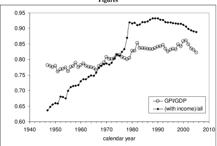
Figure 1 demonstrates the evolution of a ratio of the number of people with

income to the total working age population. There is a significant increase in this ratio:

from the lowermost value of 0.64 in 1947 to the highest 0.93 in 1988. The ratio has been

slightly decreasing since 1989 - to 0.89 in 2005. Such evolution should be definitely

reflected in the estimates of Gini coefficient – people without income introduce a large

increase in the coefficient if included. Therefore one has to consider two cases – all

population of working age and the portion with income. True PID and Gini coefficient

persons without income according to current definition, one significantly overestimates

Gini coefficient, especially in the beginning of the studied period. When only people with

income are included, Gini coefficient is underestimated. With time, these two estimates

have to converge as the portion of population without income decreases.

Second effect of the changes in income definitions and CPS procedures is related

to the change in the portion of aggregate personal income in total GDP. Introduction of

new sources of income in the CPS questionnaires should result in an increase in gross

personal income, GPI, in addition to the changes in true GPI associated with actual

processes. Figure 1 depicts the evolution of the GPI portion in the US GDP: from 0.76 in

1951 to 0.86 in 2001. A severe drop in the portion is observed between 2001 and 2005 –

from 0.86 to 0.82. The net change in the GPI portion between 1947 and 2005 is much

smaller than the change in the share of the population with income.

A fundamental assumption of the model for the evolution of individual incomes

presented in Section 1 is that all people older than 14 years have nonzero annual income

and contribute to GPI, which is equivalent to GDI and GDP in our framework. This

assumption allows modeling the PID evolution using real GDP per capita, which

completely determines time histories of the model defining parameters. The measured

PIDs are associated with a changing portion of the GDP.

In addition to the principal difficulties associated with definitions and procedures

there are some technical problems for the estimation of Gini coefficient created by the

data representation and resolution of the PIDs. The US Census Bureau provides PIDs as

the number of people enumerated in income bins of varying width. There were only 14

bins, including the open-end one for very high incomes, in 1947 and 48 bins in 2005. In

the absence of information on each and every individual income, Gini coefficient can be

calculated by some approximating relation. For example, if (Xi,Yi) are the values

obtained from the CPS, with the Xi indexed in increasing order (Xi-1 < Xi ), where Xi is

the cumulated proportion of the population variable, and Yi is the cumulated proportion

of the income variable, then the Lorenz curve can be approximated on each interval as a

straight line between consecutive points and

is the resulting approximation for G. One can also approximate the Lorenz curve using

exponential function or power law, where it is appropriate, for interpolation of the

underlying PID, as proposed by Dragulesku and Yakovenko (2001).

The choice of the appropriate function for the PID interpolation reveals an

important pitfall of the CPS - the usage of the same income bins for representation of

counted data during relatively long periods of time. The growth rate of nominal GDP in

the USA has been high - more and more people increased their incomes above the upper

income limit and found themselves in the group " $MAX and over". So, the coverage of

the populations below and above the Pareto threshold, which has been also proportionally

growing, differs by several times. This variation in the coverage might potentially result

in the increasing or decreasing overall resolution and corresponding bias in the Gini

coefficient estimation.

The US Census Bureau (2006) presents several versions of PIDs between 1947

and 2005. In some reports, tables containing PIDs in year specific income bins and

counted using current dollars are presented. Some reports give PIDs using CPI-U

adjusted (constant) or current dollars but in the same income bins for all the years staring

from 1947 to the year of the report issuance. Figure 2 shows some selected original PIDs

normalized to the total population (15 years of age and above) for corresponding years

and additionally divided by widths of corresponding income bins. Effectively, these

curves are probability density functions and show the density of population in $1-wide

bin for a given income level. Such a representation allows a direct comparison of the

PIDs because they are independent on population size and reduced to the same income

bins. As the best approximation, we associate the population density with the mean

income in a given bin. These “mean” densities obtained for bins of varying width might

be a poor approximation for the densities at the edges of the bins. The wider is the bin the

poorer is the approximation. It is worth noting that such a representation excludes the

open-end high-income bin because there is no width associated with the bin.

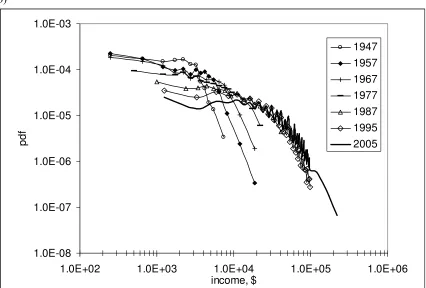
The PIDs between 1947 and 1987 shown in Figure 2a are obtained using same ten

income bins as defined by the following boundaries in current dollars: $0, $2000, $4000,

open-end bin is not shown in the Figure because it does not have finite width for

normalization of the PID reading in this bin. Thus only nine bins describe the PIDs

between 1947 and 1987.

Figure 2a illustrates the problems with resolution for constant income bins. The

PID for 1947 (and also for the years between 1948 and 1950) does not contain any

reading for incomes above $9000. This is due to the absence of the persons in

corresponding CPS samples reporting such incomes, but not because of the true absence

of such people at all. The best resolution (among the PIDs shown in the Figure) at high

incomes, i.e. in the Pareto zone, is observed in 1957 – there were seven bins covering the

zone. At the same time, there are only two bins covering the low-income zone in 1957.

For the PID in 1987, the Pareto threshold is larger than $25000, and the PID contains

only one reading in the Pareto zone corresponding to the open-end bin, i.e. the reading

not shown in the Figure. As expected, this PID provides the best resolution in the

low-income portion of the distribution – nine bins. Therefore the constant bins fail to provide

a uniform description of the PIDs between 1947 and 1987. As a result, the estimation of

Gini coefficient can be severely biased.

The PIDs between 1947 and 2005 presented in Figure 2b are characterized by

income bins which are better adjusted to the observed PIDs (US CB, 2007). These bins

cover better than in Figure 2a both low and high incomes, also with varying resolution,

however. The years after 1994 are characterized by the highest resolution, i.e. the

narrowest income bins of $2500 between $0 and $10000. Because of the increasing

number of people with incomes over $100,000, three $50000-wide bins were introduced

in 2000, covering incomes up to $250,000, extra to those provided by standard CPS

reports. These wide bins provide a more accurate representation of the Pareto distribution

and corresponding Gini coefficient.

Kitov (2005b) found that the PIDs between 1994 and 2002 practically collapse to

one curve, when normalized to the total working age population and nominal GDP per

capita – in other words to nominal GDP. (The normalized PIDs effectively represent

portion of population as a function of portion of total income.) This observation

is characterized by a fixed hierarchy of incomes, which changes slowly in time according

to the evolution of age structure.

The PIDs measured for the years before 1994 allow to validate this property and

to extend the presence of such a fixed hierarchy in the PIDs by 47 years back in the past

and 3 years ahead. There is a problem related to the normalization factor, however. The

years between 1994 and 2002 are characterized by constant values of the portions of the

GPI in the GDP and the population with income in the total working age population, as

Figure 1 demonstrates. This means that the nominal GDP grows in sync with the nominal

GPI. This is not the case for the years before 1980, however. Therefore one has to replace

the nominal GDP with nominal GPI in order to accurately represent the evolution of the

PIDs after 1947. Such a procedure has to compensate the difference in the evolution of

the GDP and GPI because less sources of personal income were considered in earlier

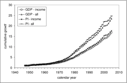
years and income scale was effectively biased down. Figure 3 displays the cumulative

growth of the nominal GDP and nominal GPI between 1960 and 2005 reduced to total

population and population with income. The curves diverge with time what allows a

more robust choice of an appropriate variable for a normalization converting all the

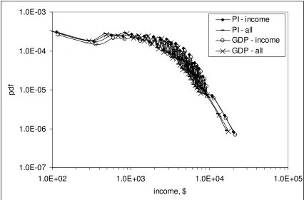
observed PIDs into one curve. Figure 4 depicts the PID for 2005 normalized to the four

variables in Figure 3. One can clearly distinguish between the resulting normalized PIDs

in the low- and high-income zones.

Figures 5 and 6 present results of the normalization of the measured PIDs to the

nominal GPI, as reduced to the people with income. For the period between 1947 and

1987 (Figure 5), where PID is measured in the same bin set, the normalized PIDs

practically collapse to one curve with only minor deviations probably associated with

measurement errors. For the period between 1947 and 2005, where a higher resolution

with varying width of income bin is available, the normalized PIDs for population with

income (Figure 6a) are also very close. The narrower bins result in higher fluctuations

due to measurement errors, however. At the same time, the normalized PIDs for all

population of 15 years of age and over demonstrate a larger divergence with time because

the normalization is associated with the nominal GPI reduced to the population with

The normalized PIDs in Figures 5 and 6a are very close. This observation extends

the presence of the fixed hierarchy of incomes, as expressed by the portion of population

having given portion of total income, to the years between 1947 and 1993, and beyond

2002. Therefore, one can expect only a slight variation in Gini coefficient related to the

PIDs. The presence of the hierarchy also represents a strong argument in favor of our

model for the evolution of individual and aggregate income.

Having studied some principal properties of the PIDs for the years between 1947

and 2005, one can start a direct estimation of Gini coefficient using the approximation

presented in (5). There are several important problems related to the discrete

representation to be resolved, however. The PIDs provide only estimates of aggregate

population but not total income in the bins. For the years after 2000, mean income is

given for each bin allowing for an accurate estimate of cumulative income. Mean

incomes are not reported for the previous years, however.

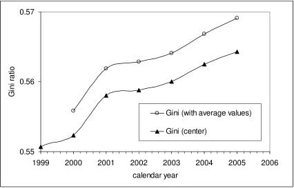
If to replace mean incomes with central points of corresponding bins, one obtains

a slightly biased value of Gini coefficient, as Figure 7 shows. Thus we need a more

reliable estimate of the mean income than provided by the central points. The best choice

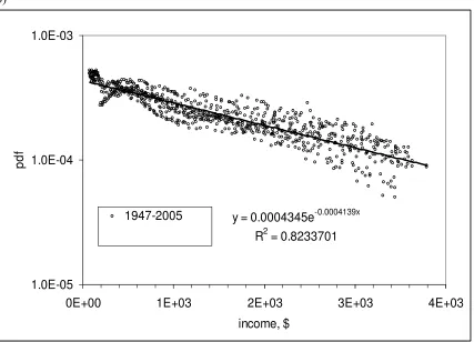
would be to approximate the observed PIDs in the low-income zone, i.e. below the Pareto

threshold, by an exponential function, to determine corresponding index for each year,

and to precisely calculate Gini coefficient for the given approximation. This approach

might potentially provide the most accurate estimate of the PIDs and Gini coefficient if

corresponding population estimates in the bins are accurate. Unfortunately, the accuracy

is inhomogeneous over the bins of varying width and the advantages of the exponential

approximation may disappear, as Figure 8 demonstrates. Therefore, we use a different

approach in the low-income zone.

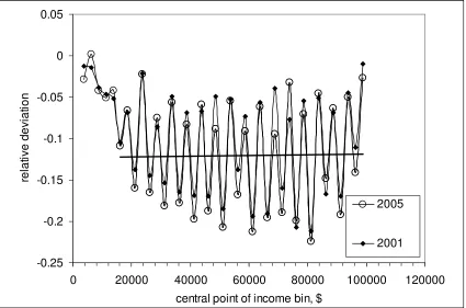
Mean income estimates are available between 2000 and 2005 and it is easy find

their average distance from the central points of relevant bins. Figure 9 presents such

deviations and corresponding regression line (mean deviation) for 2001 and 2005. The

average dimensionless distance, i.e. the difference in $ divided by the bin width in $

($2500 for the years between 2000 and 2005), is -0.12. Thus, in the following estimation

of Gini coefficient we use the mean income values corrected for this deviation in the

In the high-income zone, a power low approximation is a natural choice for the

PIDs, as demonstrated in Figures 5 and 6. Theoretically, the cumulative distribution

function, CDF, of a Pareto distribution is defined by the following relationship:

CDF(x) = 1 - (xm /x)k

for all x>xm,, where k is the Pareto index. Then, probability density function, pdf, is

defined as

pdf(x) = kxmk/x k+1 (6)

The functional dependence of the probability density function on income allows an exact

calculation of total population in any income bin, total and average income in this bin,

and the input of the bin to corresponding Gini coefficient because the pdf exactly defines

the Lorenz curve. Thus, if populations are counted in some predefined income bin set

then relevant Lorenz curve can be retrieved using a known value of the Pareto index k.

We use (6) in the following calculations of empirical Gini coefficients in the Pareto zone.

By definition, the Pareto threshold evolves proportionally to the nominal GPI per capita,

as described above. Such evolution provides the unchanged shape of the normalized PIDs

because it retains unchanged the income value where the transition from the low- to

high-income zone occurs.

Now we are ready to estimate Gini coefficients from the measured PIDs using

corrected average incomes in the low-income zone and power law approximation in the

high-income zone, the transition point evolving proportionally to the nominal GPI per

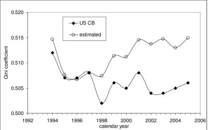
capita. To begin with, we compare our estimates of G with those reported by the US

Census Bureau, as shown in Figure 10. For the years between 1994 and 1997, the curves

are very close. In 1998, a sudden drop by ~0.01 in the CB curve is not reproduced by the

estimated one. There is no apparent reason for the drop – macroeconomic or related to the

CPS procedures. It is likely that there was some change in the US Census Bureau

slightly diverge but move in sync otherwise. The difference between the curves reaches

0.01 in 2005. Our estimates of G seem more consistent and used in further comparisons.

Figure 11 presents estimates of G for the PIDs in current dollars which do not

include people without income. There are “crude” estimates of G obtained for the

populations counted in the same income bins between 1947 and 1987. A “fine” PID is

available from the year specific bins for the period between 1947 and 2005. In spite

corresponding income bins were used several years, the overall resolution of the PIDs is

higher and G estimates are potentially of lower uncertainty. Two curves in the lower

panel of Figure 11 present the evolution of G for the two sets of PIDs – crude and fine

ones. In 1947, the curves are spaced by 0.1. When approaching 1970, they slowly

converge. Between 1974 and 1984, the curves are hardly distinguished. In 1985, a new

period of divergence starts. The observed discrepancy between the curves is related to the

coverage of the PIDs by corresponding sets of income bins.

The upper panel of Figure 11 illustrates the difference showing two Lorenz curves

for 1947. The crude set of bins does not resolve Lorenz curve well and relevant Gini

coefficient is highly underestimated as compared to the fine set. For the years between

1974 and 1984, both sets provide a compatible resolution (the number of bins is 10 and

18, respectively) and the estimates of G converge.

In fact, the Gini curve associated with the fine PIDs is a constant near 0.51

between 1960 and 2005 despite a significant increase in the GPI/GDP ratio and the

portion of people with income during this period (see Figure 1). This is a crucial

observation because of the famous discussion on the increasing inequality in the USA as

presented by the Gini coefficient for households (US CB, 2000). Obviously, the

increasing G for households reflects some changes in their composition, i.e. social

processes, but not economic processes as defined by distribution of personal incomes.

Between 1947 and 1960, the fine G curve monotonically grows from 0.45 to 0.50.

This growth may be associated with the increasing resolution in corresponding PIDs. One

can expect a further increase in the estimates of Gini coefficient when a finer grid is used.

Possibility of a slight increase in the G estimates associated with the inclusion of new

(and true) income sources is not excluded. All in all, Gini coefficient for true PIDs is

In the absence of the true PIDs one can carry out an estimate for a limit case – to

include people without income in the first bin of zero width. It is hard to believe that such

people might potentially survive, but definitions of the US CB do not allow including

income sources of the types corresponding to the incomes of people without income. In

any case, the inclusion of these people in the PIDs creates a problem for the estimation of

Gini coefficient. Figure 12 presents two time series of G estimates for the crude and fine

bin sets. In 1947, the difference is 0.04 what can be explained by the properties of

corresponding Lorenz curves, as Figure 12a depicts. Then the curves converge and

intercept in 1971. Between 1971 and 1984, the curves are very close and diverge again

since 1985. These observations are similar to those associated with the PIDs for the

population with income. The only difference is that the curves for the PIDs with total

population undergo an expected decrease with time according to the decreasing portion of

the population without income. Therefore, the Gini coefficient curves associated with the

total working age population and with its portion having nonzero income converge.

When the portion with income will reach 1.0, i.e. everybody will have has a nonzero

income, the curves become identical. So, where is our prediction relative to the empirical

curves?

3. Comparison of observed and predicted Gini indices

In the model, the evolution of personal incomes is defined by a number of parameters

which have to be determined empirically. For the estimation of Gini coefficient a critical

value is the Pareto law index, k, which defines how “thick” is the PID tail in the

high-income zone. There are two independent techniques for the estimation of k.

First, for a Pareto distribution with index k and the minimum value xm, the mean

value is

xav= (k+1)xm/k.

Therefore, the measured average incomes for the open-end income bins provide valuable

information on corresponding Pareto indices: k = xm/(xav -xm). Figure 13 presents the

available. This allows multiple estimates using the increasing number of people with

incomes above $250,000, $200,000, $150,000, and $100,000 – all in the Pareto zone. For

example, the average income for people with incomes above $100,000 in 2005 is

$176,068 and xav for people with incomes over $250,000 is $470,616. Corresponding

Pareto index values are 1.31 and 1.13. The latter estimate is obtained using the average

incomes for male and female separately, as presented by the Census Bureau. There were

10,896,000 people with income above $100,000 and only 1,334,000 above $250,000.

Bearing in mind that the population estimates are obtained using only a relatively small

sample and population controls, one can consider the Pareto index for the population with

incomes over $250,000 as less reliable than the former value. Also, the average income in

the open-end bin may be slightly shifted up due to the effect of super-rich people, who do

not obey the Pareto distribution. Such a deviation from a power law distribution is also

often in hard sciences and usually considered as statistical fluctuation related to the

under-representation in the overall population. For example, catastrophic earthquakes do

not obey Guttenberg-Richter frequency-magnitude relation. According to Figure 13,

k=1.3 is our best choice.

Second method is a direct estimation of k using regression in the Pareto income

zone. For such a regression we represent the PIDs in log-log scale as shown in Figure 14.

The power law index obtained by a linear regression is -3.35. The Pareto index is 1.35

because we use population density income distributions, i.e. the original PIDs reduced to

width of corresponding income bins. This normalization effectively increases the power

law index in the PIDs by one unit. Therefore, the Pareto index is k = 3.35-2 = 1.35 and

consistent with the results obtained by the first method.

Figure 15 demonstrates the effect of k on the predicted Gini coefficient.

Obviously, lower k values create “thicker” tails in corresponding PIDs and larger G

values. The effect of k on G is nonlinear and the difference of 0.3 units in the index value

results in Gini coefficient difference of 0.01 to 0.015. One should not neglect such a

difference when comparing predicted and measured Gini indices.

Another parameter of the model which critically depends on the Pareto index is

the effective increase in income production in the model relative to that in the sub-Pareto

corresponding ratio on k. Empirical value obtained in previous studies (Kitov, 2005a,

2005c) is 1.33. This value corresponds to k=1.35. This ratio is very sensitive to k and the

effect is also slightly nonlinear.

Having estimated the empirical parameters defining the model and the age

structure of the US population between 1947 and 2005 (US CB, 2007) one can predict

Gini coefficient (for personal incomes) during the studied period. Figure 17 compares the

measured and predicted Gini coefficients. The predicted curve is in a good agreement

with that obtained using the PIDs for the persons with income. The latter curve lies below

the former one, however, during the entire period. The empirical Gini coefficient for the

PIDs including all working age population is always above the predicted curve. Therefore

the predicted curve takes the place just between the empirical ones and the latter two

likely to converge to the predicted one in future when adequate definitions of income will

be introduced.

This is an expected result of the modeling – neither of the US Census Bureau

income definitions provides an adequate description of the personal income distribution

and thus fails to predict Gini coefficient. Usage of such biased G values may lead to

economic misinterpretation and social confusion. The Gini coefficient for personal

incomes in the USA underwent a slight increase between 1947 (0.5346) and 1962

(0.5378), and then has been monotonically decreasing to the current value of 0.524.

There was no significant increase in the economic inequality in the USA during the last

60 years as expressed by the Gini coefficient for personal incomes.

4. Conclusion

There are several simple but meaningful findings related to the estimation of the

empirical Gini coefficients. First and most important consists in the fact that the estimates

of Gini coefficient critically depend on definition of income. The inclusion of new

income sources in the CPS questionnaires has resulted in a large change in the number of

people with income and also in the ratio of GPI and GDP. The current set of definitions is

far from that necessary for measuring true PIDs, however.

Second, the Gini coefficient associated with whole population 15 years of age and

portion of people without income decreases. The true Gini coefficient had to be

somewhere between these two estimates. Thus the empirical estimates can not be

considered as reliable for the purposes of economics as a theory.

Third, the resolution of the empirical PIDs, i.e. the coverage of population with

income bins in some proportional ways, influences the estimates of Gini coefficient. A

higher resolution guarantees a smaller variation in Gini coefficient over time. Poor

resolution leads to a negative bias in the G estimates.

Fourth, the empirical PIDs collapse to practically one curve when normalized to

the cumulative growth in nominal GPI for the studied period between 1947 and 2005.

The remaining differences in the PIDs are well reflected in the changes of the Gini

coefficient obtained using the population with income. The empirical PIDs support the

assumptions of the model for the evolution of individual income.

The model predicts practically unchanged (normalized) PIDs and Gini coefficient

between 1947 and 2005. Slight changes in the PIDs and G are related to economic growth

and changes in the age structure of American population. The decreasing portion of

young and thus relatively low-paid people in the working age population effectively leads

to a decrease in Gini coefficient. The increasing portion of the population older than the

critical age Tcr (55 years in 2005) results in an increase in the portion of relatively poor

people because of the exponential decrease of income (including average one) with age,

as described in Section 1. As a net result of the two effects, the empirical Gini coefficient

has a minimum of 0.5238 in 1990 and then starts to grow again, reaching 0.5266 in 2005.

Such defining model parameters as the Pareto law index (1.35) and the ratio of the

efficiency of money earning in the Pareto zone relative to the predicted by the model

(1.33) are well calibrated by the empirical PIDs and Gini coefficient. The model for the

individual income evolution is very sensitive to these parameters.

The empirical Gini curves converge to the predicted one when the number of

people without income according to currently adopted definitions decreases.

Asymptotically, the empirical curves should collapse to the theoretical one when all the

working age population will obtained an appropriate definition of their incomes. Such

convergence should be seen clearly in age dependent PIDs, where the portion of the

and 54 years this portion increased from 0.78 in 1960 to 0.94 in 2005. Hence, the portion

was consistently larger and changed less than that for the total working age population

(see Figure 1). One can expect a lower difference between the two empirical estimates

and a better prediction. This is a subject of a paper in preparation.

Gini coefficient is a crude and secondary measure of inequality for economics as

a science. It could be useful for social and political discussions as a relative and

operational measure without any specific meaning of its absolute value. What is

important and has a primary significance for scientific models are the PIDs, which

demonstrate a fixed hierarchy during a very long period between 1947 and 2005. (It is

very unlikely that this hierarchy will be destroyed in near future.) The shape and the

evolution of the measured PIDs is well predicted for the whole period between 1947 and

2005. This allows exact prediction of the Gini coefficient and other measures of

inequality, which are defined using personal income distribution.

The Census Bureau focuses its attention on Gini coefficients related to the

measurements of income inequality at family and household level. Corresponding

coefficients change with time and are presented as evidence in favor of an increasing

economic inequality in the USA (US CB, 2000). Our estimates of the Gini coefficient for

the PIDs, both empirical and theoretical, demonstrate that the inequality is not changing

so dramatically. Therefore the Gini coefficient associated with households should be

affected primarily by some changes in their structure but not by the changes in the

References

Dragulesky, A., and Yakovenko, V. (2001). Exponential and power-law probability distributions of wealth and income in the United Kingdom and the United States. Physica A: Statistical Mechanics and its Applications, 299, 1-2 , 213-221

Kitov, I. (2005a). A model for microeconomic and macroeconomic development. Working Paper 05, ECINEQ, Society for the Study of Economic Inequality. Kitov, I. (2005b). Modeling the overall personal income distribution in the USA from

1994 to 2002. Working Paper 07, ECINEQ, Society for the Study of Economic Inequality

Kitov, I. (2005c). Evolution of the personal income distribution in the USA: High

incomes. Working Paper 02, ECINEQ, Society for the Study of Economic Inequality

Kitov, I. (2006a). Modeling the age-dependent personal income distribution in the USA.

Working Paper 17, ECINEQ, Society for the Study of Economic Inequality Neal, D. and Rosen, S. (2000). Theories of the distribution of earnings. In: Handbook of

Income Distribution, (Eds.) Atkinson, A. and Bourguinon, F., 379-427, Elsevier 2000.

Rodionov, V.N., Tsvetkov, V.M., and Sizov, I.A. (1982). Principles of Geomechanics. Nedra, Moscow, p.272. (in Russian)

U.S. Census Bureau. (2000). The Changing Shape of the Nation's Income Distribution. Retrieved February 26, 2007 from http://www.census.gov/prod/2000pubs/p60-204.pdf

U.S. Census Bureau. (2002). Technical Paper 63RV: Current Population Survey - Design and Methodology, issued March 2002. Retrieved February 26, 2007 from http://www.census.gov/prod/2002pubs/tp63rv.pdf

US Census Bureau. (2006). Current Population Reports. Consumer Income Reports from 1946-2005. (P60). Retrieved March 14, 2007 from http://www.census.gov/prod/ www/abs/income.html)

US Census Bureau. (2007). Population Estimates. Retrieved March 14, 2007 from http://www.census.gov/popest

Figures

0.60 0.65 0.70 0.75 0.80 0.85 0.90 0.95

1940 1950 1960 1970 1980 1990 2000 2010

calendar year

GPI/GDP (with income)/all

a)

1.0E-07 1.0E-06 1.0E-05 1.0E-04 1.0E-03

1.0E+02 1.0E+03 1.0E+04 1.0E+05

income, $

p

d

f

b)

1.0E-08 1.0E-07 1.0E-06 1.0E-05 1.0E-04 1.0E-03

1.0E+02 1.0E+03 1.0E+04 1.0E+05 1.0E+06

income, $

p

d

f

1947 1957 1967 1977 1987 1995 2005

Figure 2. PIDs for selected years measured in current dollars: a) – for the years between 1947 and 1987 in constant income bins; b) – for the years between 1947 to 2005 in varying income bins. The PIDs are normalized to the total population and reduced to width of corresponding income bin.

0 5 10 15 20 25 30

1940 1950 1960 1970 1980 1990 2000 2010

calendar year

c

u

m

u

la

ti

v

e

g

ro

w

th

GDP - income GDP - all PI - income PI - all

1.0E-07 1.0E-06 1.0E-05 1.0E-04 1.0E-03

1.0E+02 1.0E+03 1.0E+04 1.0E+05

income, $

p

d

f

PI - income PI - all

GDP - income GDP - all

1.0E-07 1.0E-06 1.0E-05 1.0E-04 1.0E-03

1.0E+02 1.0E+03 1.0E+04 1.0E+05

income, $

p

d

f

1947 1957 1967 1977 1987

a)

1.0E-07 1.0E-06 1.0E-05 1.0E-04 1.0E-03

1.0E+02 1.0E+03 1.0E+04 1.0E+05

income, $

p

d

f

b)

1.0E-07 1.0E-06 1.0E-05 1.0E-04 1.0E-03

1.0E+02 1.0E+03 1.0E+04 1.0E+05

income, $

p

d

f

1995 1987 1967 1977 1947 1957 2005

0.55 0.56 0.57

1999 2000 2001 2002 2003 2004 2005 2006

calendar year

G

in

i

ra

ti

o

Gini (with average values)

Gini (center)

a)

y = 0.0004213e-0.0003991x R2 = 0.9368865

1.0E-05 1.0E-04 1.0E-03

0.0E+00 1.0E+03 2.0E+03 3.0E+03 4.0E+03

income, $

p

d

f

b)

y = 0.0004345e-0.0004139x

R2 = 0.8233701

1.0E-05 1.0E-04 1.0E-03

0E+00 1E+03 2E+03 3E+03 4E+03

income, $

p

d

f

1947-2005

-0.25 -0.2 -0.15 -0.1 -0.05 0 0.05

0 20000 40000 60000 80000 100000 120000

central point of income bin, $

re

la

ti

v

e

d

e

v

ia

ti

o

n

2005

2001

Figure 9. Relative deviation of the average value in income bins, Xav, from the central

point of the bin, Xc : (Xav-Xc)/dX, where dX is the width of corresponding bin. The CPS

0.500 0.505 0.510 0.515 0.520

1992 1994 1996 1998 2000 2002 2004 2006

calendar year

G

in

i

c

o

e

ff

ic

ie

n

t

US CB

estimated

a)

0.0 0.2 0.4 0.6 0.8 1.0

0.0 0.2 0.4 0.6 0.8 1.0

crude 1947

b)

0.30 0.35 0.40 0.45 0.50 0.55

1940 1950 1960 1970 1980 1990 2000 2010

calendar year

G

in

i

c

o

e

ff

ic

ie

n

t

Gini - with income (1947-2005)

Gini - with income (1947-1987)

a)

0.0 0.2 0.4 0.6 0.8 1.0

0.0 0.2 0.4 0.6 0.8 1.0

b)

0.5 0.52 0.54 0.56 0.58 0.6 0.62 0.64 0.66

1940 1950 1960 1970 1980 1990 2000 2010

calendar year

G

in

i

co

e

ff

ic

ie

n

t

Gini - all (1947-2005) Gini - all (1947-1987)

0 0.2 0.4 0.6 0.8 1 1.2 1.4 1.6

1 3 5 7 9 11 13 15 17 19 21 23

Figure 13. Estimates of the power law index k obtained from the average values of

y = 2.83E+08x

1.0E-07 1.0E-06 1.0E-05 1.0E-04

1.0E+03 1.0E+04 1.0E+05

income

p

d

f/

in

c

o

m

e

Figure 14. Linear regression of the normalized PIDs in the Pareto zone (log-log

coordinates). The Pareto index is k=1.36. This estimate is consistent with that obtained

using the average values above $100000 in Figure 13. Notice that the PIDs are divided by income bin widths in order to obtain density function independent on the widths. This