A Five Step P Stable Method for the Numerical Integration of Third Order Ordinary Differential Equations

(1)

http://dx.doi.org/10.4236/ajcm.2014.43011

A Five-Step P-Stable Method for the

Numerical Integration of Third Order

Ordinary Differential Equations

D. O. Awoyemi

1

_{, S. J. Kayode}

2

_{, L. O. Adoghe}

3

1_{Department of Mathematics, Landmark University, Umuaru, Nigeria}

2_{Department of Mathematical Sciences, Federal University of Technology, Akure, Nigeria} 3_{Department of Mathematics, Ambrose Alli University, Ekpoma, Nigeria}

Email: [email protected]

Received 26 December 2013; revised 26 February 2014; accepted 6 March 2014

This work is licensed under the Creative Commons Attribution International License (CC BY).

http://creativecommons.org/licenses/by/4.0/

Abstract

In this paper we derived a continuous linear multistep method (LMM) with step number k = 5 through collocation and interpolation techniques using power series as basis function for ap-proximate solution. An order nine p-stable scheme is developed which was used to solve the third order initial value problems in ordinary differential equation without first reducing to a system of first order equations. Taylor’s series algorithm of the same order was developed to implement our method. The result obtained compared favourably with existing methods.

Keywords

Continuous Collocation, Multistep Methods, Interpolation, Third Order, Power Series, Approximate Solution

1. Introduction

Linear multistep methods (LMM) for solving first order initial value problems (ivps) is of the form

0 0

k k

j n j j n j

j y hj f

α ₊ β ₊

= =

=

∑

(1)

where

α

j and

β

j are uniquely determined and α0+βj≠0,αk =1

(2)

a system first order has some serious drawback which includes wastage of human effort and computer time [6]. The LMM in (1) generates discrete schemes which are used to solve first order odes. Various forms of this LMM have been developed [1]-[4]. Other researchers have introduced the continuous LMM using the continuous collocation and interpolation technique. This has led to the development of continuous LMM of form

( )

0 0

k k

j n j j n j

j j

Y x α t y+ h β t f +

= =

=

∑

+

∑

(2)

j

α

and

β

j are expressed as continuous functions of t and are at least differentiable once.

The introduction of continuous collocation methods as against the discrete schemes enhances better global error estimation and ability to approximate solution at all interior points [6]-[10]. In this study, we shall develop con-tinuous multistep collocation method for the solution of third order ordinary differential equations using power series as the basis function.

Power Series Collocation

In [6] [8] [9], some continuous LMM of Type (2) were developed using power series of form

( )

0

k j j j

Y x a x

=

∑

: (3)

In [10] Chebyshev polynomial function of the form

( )

0 k

k j j

j

x x Y x a T x

h

=

−

 

= _ _

 

∑

(4)

where T xj

( )

are some Chebyshev function used to develop continuous LMM.

The use power series as basis function for derivation of continuous LMM are based on the property of analytic function that given the Taylor’s polynomial of the form

( )

( )(

0

)

0 !

r n

n

r

y x x x P x

r

=

−

=

∑

(5)

The approximate function p x

( )

reduces to Y x

( )

as n→ ∞ In this study we proposed the polynomial function of the form in [7]:

( )

(

)

0

k _j

j n

j

Y x a x x

=

∑

− (6)

which is of Type (3) to develop a continuous LMM for the solution of initial value problem of the form:

(

, , ,

) ( )

, 0;

( )

0,

( )

N

y′′′= f x y y y y a′ ′′ =y y a′ = ∂ y a′′ = ∂ (7) This paper is organized as follows: Section 1 consists of introduction and background of study; Section 2, we derive a continuous approximation to Y x

( )

for exact solution y x

( )

, and specific methods; Section 3 consists of the analysis and implementation followed by numerical examples.

2. Derivation of

the Method

Consider the third order differential Equation (7), we proposed an approximate solution of the form:

( )

0

M

k j j

j

y x aψ x

=

∑

(8)

where ψj

( )

x =

(

x x− n

)

j,j≥0.

The derivative of (8) up to the third order yield

( )

(

)(

)

3

( )

0 1 2

k

k j j

j

y x j j j aψ ₋ x

=

(3)

And a x b≤ ≤ where a s′j are the parameters to be determined. By substituting (8) and (9) into (7) we have

(

)(

)

3

( )

(

)

0 1 2 , , ,

k

j j

j j j j a x f x y y y

ψ − =

′ ′′

− − =

∑

(10)

Collocating (10) at x x= n i+,i=0 1

( )

m and interpolating (8) at x x= n i+,i=0 1

( )

m−1 we obtained the system of equations given below

(

)

0

M

j j n i n i

j a x y

ψ ₊ ₊

=

∑

(11)

(

)(

)

3

( )

0 1 2

M

j j n i

j j j j a x f

ψ ₋ ₊

=

− − =

∑

(12)

The above equations are solved to obtain the values of a s′j which when substituted into Equation (6) yield a

method of the form in Equation (13)

( )

1

( )

0 0

k k

j n j j n j

j j

Y x −α t y+ h β t f+

= =

=

∑

+

∑

(13)

The continuous polynomial obtained when the values of a s′j are substituted into (6) and simplified is as

follows

( )

(

)

(

)

(

)

(

)

(

)

(

)

(

)

(

)

(

)

(

)

(

)

2 4

10 9 8 6

10

5 6 8

5 4 3 7 2

9 10

2

9 8

10

1 ₅₉₅₂₀ _3305158 _5968895 _8146800

59520

8869224 4685898 1424760 253425

24490 1024

1 _6211314 _11400365 _1562776

59520

n n n

n n n n

n n n

n n

Y x h h x x h x x h x x

h

h x x h x x h x x h h x x

h x x x x y

h x x h x x

h  = _ − − + − − − + − − − + − − −  + − − − _ + − − − +

(

)

(

)

(

)

(

)

(

)

(

)

(

)

(

)

(

)

(

)

(

)

(

)

(

)

4 6

5 6 7 8

5 4 3 2

9 10

1

2 4 5

9 8 6 5

10

6 7

4 3

00

17084088 9069483 2770920 495075

48030 1952

1 ₈₉₈₀₆₂ ₁₅₈₂₅₁ ₁₉₉₈₀₀ _1963080

59520

907074 235800 3532

n

n n n n

n n n

n n n n

n n

h x x

h x x h x x h x x h x x

h x x x x y

h x x h x x h x x h x x

h

h x x h x x

+  ₋  − − + − − − + −  − − + − _  + _ − − − + − − − + − − − +

(

)

(

)

(

)

(

)

(

)

(

)

(

)

(

)

(

)

(

)

(

)

(

)

8 9 10

2

2 4

9 8 6

10

5 6 7 8

5 4 3 2

9 10

3

7

5 2850 96

1 _7311962 _13490545 _18291600

59520

19701528 10278870 3085320 542175

51830 2080

1 ₁₆₀₁

399974400

n n n n

n n n

n n n n

n n n

h x x h x x x x y

h x x h x x h x x

h

h x x h x x h x x h x x

h x x x x y

h + +  − − − + − _  + _− − + − − − + − − − + − − −  + − − − _ + −

(

)

(

)

(

)

(

)

(

)

(

)

(

)

(

)

(

)

(

)

(

)

2 3

9 8 7

4 5 6 7

6 5 4 3

8 9 10

2

9 7

64924 27846271 6666240

50359720 518336784 269004260 81125040

14366570 98910 56000

1 _9863776238 _18418906560

399974400

n n n

n n n n

n

h x x h x x h x x

h x x h x x h x x h x x

h x x h x x x x f

h x x h

h  ₋ ₊ ₋ ₊ ₋  − − + − − − + −   − − + − _− − __ + − − +

(

)

(

)

(

)

(

)

(

)

(

)

(

)

(

)

2 4 8 6

5 6 7

5 4 3

8 9 10

2

1

25437064780

27743628290 14672416610 4463635120

794196650 5482910 3109568

n n

n n n

n n n n

x x h x x

h x x h x x h x x

h x x h x x x x f +

 ₋ ₋ ₋



+ − − − − −



(4)

(

)

(

)

(

)

(

)

(

)

(

)

(

)

(

)

(

)

2 4

9 8 6

7

5 6 7

5 4 3

8 9 10

2

7

1 _2355609311 _43809648630 _59823556780

399974400

64857656850 34104473030 10321466720

1828259700 12572860 7107968

1 ₁₀₉₆₉₇

399974400

n n n

n n n n

h x x h x x h x x

h

h x x h x x h x x

h x x h x x x x f

h +  + _− − + − − − + − − − + −  + − + − − − _ + −

(

)

(

)

(

)

(

)

(

)

(

)

(

)

(

)

(

)

(

)

2 4

9 8 6

5 6 5

5 4 5

8 9 10

2

3

9 8

7

70700 20392494160 27749220780

29987527570 157505754790 4732439520

834535300 5715660 3219328

1 _177230988 _329512510

399974400

n n n

n n n n

n

h x x h x x h x x

h x x h x x x x f

h x x h

h +  ₋ ₊ ₋ ₋ ₋  + − − − + −  + − + − − − _ + − − +

(

)

(

)

(

)

(

)

(

)

(

)

(

)

(

)

(

)

(

)

(

)

(

)

2

4 5 6

6 5 4

7 8 9 10

3 2

4

2 4 5

9 8 6 5

7

449080800 486136784 255405332

77358320 13746850 95110 54208

1 _2399724 _4458670 _5990880 _6383440

399974400 36208

n

n n n

n n n n n

n n n n

x x

h x x h x x h x x

h x x h x x h x x x x f

h x x h x x h x x h x x

h +  ₋  − − + − − −  + − + − + − − − _  + _− − + − − − + −

− 4

(

)

6 3

(

)

7 2

(

)

8

(

)

9

(

)

10

5 52h x x− n +941680h x x− n −154930h x x− n +950h x x− n −448 x x− n _fn+

(14) Evaluating (14) at x x= n+5 the following discrete method is obtained

5 4 3 2 1

3

5 4 3 2 1

29 68 68 29

31 31 31 31

21 1177 1921 1921 1177 21

2480 2480 1240 1240 2480 2480

n n n n n n

y y y y y y

h f f f f f f

+ + + + + + + + + + − − + + −   = _ + + + + + _   (15)

3. Analysis and Implementation of the Method

3.1. Basic Properties of the Method

The method (15) is a specific member of the conventional LMM which can expressed as

3

0 0

k k

j n j j n j

j y h j y

α + β +

= =

′′′ =

∑

(16)

Following [1] [2], we define the local truncation error associated with (16) by the difference operator

( )

(

)

3

(

)

0

; k j n j n

j

L y x h α y x jh h β y x jh

=

 ′′′ 

= + − +

 

 

∑

  (17)

where y x

( )

is assumed to have continuous derivatives of sufficiently high order. Therefore expanding (23) in Taylor series about the point x to obtain the expression

( )

1 1

( )

2 2

( )

0 1 2 1 2

; p p p p P p

p p p

L y x h C y x C hy x C hy x C h y x C h y+ + x C h y+ + x

+ +

′ ′′

= + + + + + +

 

   (18)

where the C C C0, , , ,1 2 Cp+2 are defined as

0 0 k j j C α =

=

∑

, 1 0

k j j

C jα

=

∑

, 2

2 1 1 2! k j j

C jα

=

∑

,

(

)(

)

3

1 1

1 ₁ ₂

!

k k

q q

q j j

j j

C j q q q j

q α β

−

= =

 

= _ − − − _



∑



In the sense of [1], we say that the method (20) is of order p and error constant Cp+2 ≠0 if

0 1 2 p 1 0, p 2 0

C =C C= ==C + = C + ≠

(5)

2 0.005403 2

p p

C + = − C +

3.2. Zero-Stability of the 5-Step Method

Considering the first characteristics polynomial of the method of Equation (15) given as

( )

5 29 4 68 3 68 2 29 _{1 0}

31 31 31 31

r r r r r r

ρ = − − + + − =

Putting r=1,

ρ

( )

r =0 implying that r−1 is a factor. Therefore solving the polynomial it is found that

(

)

3

1

r− is also a factor of the polynomial and r=1,1,1. The other roots which are called spurious roots are 0.776216472

r= − and −1.28829956.

3.3. Region of Absolute Stability of the 5-Step Scheme

Applying the boundary locus method, we have that

( )

5 29 4 68 3 68 2 29 _{1 0}

31 31 31 31

r r r r r r

ρ = − − + + − =

( )

3

(

₂₁ 5 ₁₁₇₇ 4 ₃₈₄₂ 3 ₃₈₄₂ 2

( )

₁₁₇₇ ₂₁

)

2480

h

r r r r r r r

σ = + + + σ + +

In the spirit of Lambert (1973),

( )

_{( )}

( )

i

i e e r h r

r

θ

θ ρ ρ

σ σ

= =

By letting _r₌_eiθ ₌_cos_θ₊_isin_θ_{and substituting this into the express above to yield}

( )

2480 cos5

{

29cos 4 68cos3 68cos 2 29cos 1

}

21cos5 1177cos 4 3842cos3 3842cos 2 1177cos

x θ θ θ θ θ θ

θ θ θ θ θ

− − + + +

=

+ + + +

At θ =0_and_{θ =}₁₈₀

for 0≤ ≤θ 180 at an interval of 30 we have that X

( ) (

θ

= 0,∞

)

. The method is therefore said to be p-stable.

3.4. Implementattion

Single step method can be used to solve higher order ordinary differential equations directly without the need to first reducing it to an equivalent system of first order.

Consider the initial value problem in (7). For our method of order p=9, Taylor series expansion is used to calculate.

1, 2, 3

n n n

y+ y+ y+ and their first, second, third derivatives up to order p=9.

(

)

( )

( ) ( )

( )

2 3 4

5 6 7 8 9

2! 3! 4!

5! 6! 7! 8! 9!

1 1 4

n j n

n n n

n n

iv v vii

n n n n n

y y x jh

jh y x jh f jh f y x jhy x

jh f jh f jh f jh f jh f

j

+ ≡ +

′′ ′

′

≅ + + + +

′′ ′′′

+ + + + +

=

(

)

( )

( ) ( )

( )

2 3 4 5 6

7 8 9

2! 3! 4! 5! 6!

7! 8! 9!

iv

n n n n n

n j n n n

v vi vii

n n n

y y x jh y x jhy x

jh f jh f jh f

+

′ ′′ ′′′

′ ≡ ′ + ≅ ′ + ′′ + + + + +

(6)

(

)

( )

2 3

4 5 6 7 8 9

2! 3!

4! 5! 6! 7! 8! 9!

n j n

n n

iv v vi vii viii

n n n n n n

y y x jh

jh f jh f

y x jhf

jh f jh f jh f jh f jh f jh f

+

′′ ≡ ′′ +

′ ′′

′′

≅ + + +

′′′

+ + + + + +

(

)

( )

2 3 4

5 6 7 8 9

2! 3! 4!

5! 6! 7! 8! 9!

n j n

iv

n n n

n n

v vi vii viii ix

n n n n n

y y x jh

jh f jh f jh f

f jhf

+

′′′ ≡ ′′′ +

′′ ′′′

′

≅ + + + +

+ + + + + +

Then the known values of xn and yn are substituted into the differential equations. Next the differential

equation is differentiated to obtain the expression for higher derivatives using partial differentiation as follows

(

, , ,

)

j

y′′′= f x y y y′ ′′ = f

iv

x y y y j

y f y f y f ff y y f Df

x y y y

′ ′′

 ∂ ∂ ∂ ∂ 

′ ′′ ′ ′′

= + + + =_ + + + _=

′ ′′

∂ ∂ ∂ ∂

 

( )

( ) (

)

( )

(

)

( )

(

)

2 2 ₂

2 2

2 2 2

v

xx yy y y y y xy xy xy

yy yy y y j y j y

j y j j y _j j y j j y _j

y f y f y f f f y ff y f ff

y y f y ff y ff Df f f y f

D f f Df f y f D f f Df f y f

′ ′ ′′ ′′ ′ ′′

′ ′′ ′ ′′ ′ ′

′′ ′ ′′ ′

′ ′′ ′ ′′

= + + + + + +

′ ′′ ′ ′′ ′′

+ + + + + +

′′ ′′

= + + + = + + +

where

D y y f

x y y y

 ∂ _′ ∂ _′′ ∂ ∂ 

=_ + + + _

′ ′′

∂ ∂ ∂ ∂

  and

( )

2

D =D D

P j

D f where p is the order of the method.

3.5. Numerical Experiments

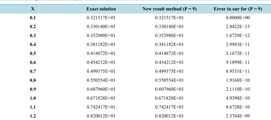
Our methods of order p=9 were used to solve some initial value problems of both general and special nature using Taylor’s series. Our results were compared with the results of other researchers in this area as seen in Table 1. In Table 2 and Table 3, the accuracy of our method is seen in the small error values.

The following initial value problems were used as our test problems:

3.6. Problem 1

( )

, 0 1, 0 1, 0 1.

1, 0.1

y y y y y

o x h

′′′= − = ′ = − ′′ =

≤ ≤ =

Exact solution: _{y x}

( )

₌e−x_.

3.7. Problem 2

( )

2 2 2

. 2 3 10 34 e 16e 10 6 34.

0 3, 0 0, 0 0,0 1

x x

y y y y x x x

y y y x

− −

′′′− ′′− ′+ = − − + +

′ ′′

= = = ≤ ≤

(7)

3.8. Problem 3

ex

y′′′ = , y

( )

0 =3,y′

( )

0 1,= y′′

( )

0 =5 Exact solution: _{2 2}₊ _x2₊_ex

[image:7.595.88.538.166.316.2]

.

Table 1. Showing the result of test problem 1.

X Exact solution New result method (P = 9) Error in our for (P = 9) Error in [11] (P = 9)

0.1 0.904837 0.940837 0.0000+00 2.1760E−12

0.2 0.818731 0.818731 2.7756E−14 1.3935E−11

0.3 0.740818 0.740818 1.5838E−12 3.4443E−11

0.4 0.670320 0.670320 2.7879E−11 6.4477E−11

0.5 0.606531 0.606531 2.9477E−11 1.0316E−10

0.6 0.548812 0.548812 8.5048E−11 1.4979E−10

0.7 0.496585 0.496585 8.0357E−11 2.0486E−10

0.8 0.449329 0.449329 1.6601E−10 2.6756E−10

0.9 0.406570 0.406570 1.1176E−10 6.9382E−10

1.0 0.367879 0.367879 1.4871E−10 1.4224E−10

X Exact solution New result method (P = 9) Error in our for (P = 9)

0.1 0.299819E+01 0.299819E+01 6.6218E−13

0.2 0.298681E+1 0.298681E+01 6.2238E−11

0.3 0.295939E+01 0.295939E+01 3.5134E−09

0.4 0.291189E+01 0.291189E+01 6.1100E−07

0.5 0.284197E+01 0.284197E+01 6.4183E−07

0.6 0.274843E+01 0.274843E+01 1.8082E−06

0.7 0.263083E+01 0.263083E+01 1.3511E−06

0.8 0.248921E+01 0.248921E+01 1.3367E−06

0.9 0.232389E+01 0.232390E+01 7.9041E−06

1.0 0.213534E+01 0.213537E+01 3.7360E−05

X Exact solution New result method (P = 9) Error in our for (P = 9)

0.1 0.321517E+01 0.321517E+01 0.0000E+00

0.2 0.330140E+01 0.330140E+01 2.8422E−13

0.3 0.352980E+01 0.352980E+01 1.6729E−12

0.4 0.381182E+01 0.381182E+01 2.9983E−11

0.5 0.414872E+01 0.414872E+01 3.1673E−11

0.6 0.454212E+01 0.454212E+01 9.1899E−11

0.7 0.499375E+01 0.499375E+01 8.9531E−11

0.8 0.550554E+01 0.550554E+01 1.9168E−10

0.9 0.607960E+01 0.607960E+01 2.1110E−10

1.0 0.671828E+01 0.671828E+01 4.9398E−10

1.1 0.742417E+01 0.742417E+01 8.6728E−10

[image:7.595.90.537.522.720.2]

(8)

4. Discussion of Result

We have developed and implemented our methods using Taylor series of the same order as the schemes that we developed. Some special and general third order initial value problems (ivps) were used to test the efficiency of our methods. Our method was found to be zero stable, consistent and convergent. The better accuracy of our method can be shown from the numerical examples.

References

[1] Lambert, J.D. (1973) Computional Methods in ODEs. John Wiley & Sons, New York.

[2] Fatunla, S.O. (1988) Numerical Methods for Initial Value Problems in Ordinary Differential Equations. Academic Press Inc., Harcourt Brace, Jovanovich Publishers, New York.

[3] Butcher, S.C. (2003) Numerical Methods for Ordinary Differential Equations. John Wiley & Sons, New York. http://dx.doi.org/10.1002/0470868279

[4] Henrici, P. (1962) Discrete Variable Method in Ordinary Differential Equations. John Wiley & Sons, New York. http://dx.doi.org/10.1002/zamm.19660460521

[5] Bruguano, L. and Trigiante. D. (1998) Solving Differential Problems by Multistep Initial and Boundary Value Methods. Gordon and Breach Science Publishers, Amsterdam, 280-299.

[6] Awoyemi, D.O. (2003) A P-Stable Linear Multistep Method for Solving General Third Order Ordinary Differential Equations. International Journal of computer Mathematics, 80, 987-993.

http://dx.doi.org/10.1080/0020716031000079572

[7] Okunuga, S.A. and Ehijie, J. (2009) New Derivation of Continuous Multistep Methods Using Power Series as Basis Function. Journal of Modern Mathematics and Statistics, 3, 43-55.

[8] Adesanya, A.O. (2011) Block Methods for Direct Solutions of General Higher Order Initial Value Problems of Ordi-nary Differential Equations. Ph.D. Thesis, the Department of Mathematical Sciences, Federal University of Technolo-gy, Akure.

[9] Adeniyi, R.B. and Alabi, M.O. (2006) Derivation of Continuous Multistep Methods Using Chebyshev Polynomial Ba-sis Functions. Abacus, 33, 351-361.

[10] Onumanyi, P., Oladele, J.O., Adeniyi, R.B. and Awoyemi, D.O. (1993) Derivation of Finite Difference Method by Collocation. Abacus, 23, 2-83.