S e q u e n ti al r e g r e s si o n
m e a s u r e m e n t e r r o r m o d e l s wi t h
a p p li c a ti o n
S c a rf, PA a n d M off a t t , JL
h t t p :// dx. d oi.o r g / 1 0 . 1 1 7 7 / 1 4 7 1 0 8 2X 1 6 6 6 3 0 6 5
T i t l e S e q u e n ti al r e g r e s sio n m e a s u r e m e n t e r r o r m o d el s wi t h a p p lic a ti o n
A u t h o r s S c a rf, PA a n d M off a t t, JL
Typ e Ar ticl e
U RL T hi s v e r si o n is a v ail a bl e a t :
h t t p :// u sir. s alfo r d . a c . u k /i d/ e p ri n t/ 3 9 9 7 7 /
P u b l i s h e d D a t e 2 0 1 6
U S IR is a d i gi t al c oll e c ti o n of t h e r e s e a r c h o u t p u t of t h e U n iv e r si ty of S alfo r d . W h e r e c o p y ri g h t p e r m i t s , f ull t e x t m a t e r i al h el d i n t h e r e p o si t o r y is m a d e f r e ely a v ail a bl e o nli n e a n d c a n b e r e a d , d o w nl o a d e d a n d c o pi e d fo r n o
n-c o m m e r n-ci al p r iv a t e s t u d y o r r e s e a r n-c h p u r p o s e s . Pl e a s e n-c h e n-c k t h e m a n u s n-c ri p t fo r a n y f u r t h e r c o p y ri g h t r e s t r i c ti o n s .
Sequential regression measurement error models
with application
Joanne L Moffatt1and Phil Scarf2
1School of Computing Science and Engineering, University of Salford, Salford, UK
2Salford Business School, University of Salford, Salford, UK
Abstract: Sequential regression approaches can be used to analyze processes in which covariates are revealed in stages. Such processes occur widely, with examples including medical intervention, sports contests and political campaigns. The na¨ive sequential approach involves fitting regression models using the covariates revealed by the end of the current stage, but this is only practical if the number of covariates is not too large. An alternative approach is to incorporate the score (linear predictor) from the model developed at the previous stage as a covariate at the current stage. This score takes into account the history of the process prior to the stage under consideration. However, the score is a function of fitted parameter estimates and, therefore, contains measurement error. In this article, we propose a novel technique to account for error in the score. The approach is demonstrated with application to the sprint event in track cycling and is shown to reduce bias in the estimated effect of the score and avoid unrealistically extreme predictions.
Key words: logistic regression; measurement error; sequential regression; staged processes; track cycling
ReceivedJanuary 2015;revisedJanuary 2016;acceptedJuly 2016
1 Introduction
Consider a stochastic control process or prediction problem in which a random outcome depends on a set of non-random covariates such that (a) disjoint subsets of the covariates are revealed in stages and (b) at each stage, a model (explanatory or predictive) for the outcome is required. Such processes, which have a natural order given by the discretization of time into stages, occur in many fields: for example, medics may wish to model patient survival prior to intervention, immediately post intervention, and prior to discharge taking account of patient, disease and interven-tion characteristics revealed at each stage; in a sporting context, coaches and players would like to understand the effect of tactical decisions on overall outcome as the contest progresses; and politicians may wish to assess the effectiveness of tactics used during various stages of a political campaign. At each stage, a vector of covariates is revealed, and a modeller/statistician might take one of the following approaches:
Address for correspondence: Joanne L Moffatt, School of Computing Science and Engineering, University of Salford, Salford, M5 4WT, UK.
1. At each stage i= 1, ..., m, fit a model that contains the covariates revealed up to and including stage i, repeating this process at each stage (na¨ive sequential regression).
2. At the first stage, fit a model that contains the covariates revealed at the first stage, and then at each stagei=2, ..., m, fit a model that contains the covariates revealed at stage iplus the estimated linear predictor from the previous stage
i−1. Elisheva et al. (2000) refer to models, obtained in this way as sequential models and we will follow their convention of referring to the linear predictor as the score throughout this article.
The na¨ive approach (1) may be practical if both the total number of covariates and the number of stages are not too large. Otherwise, we should anticipate difficulties regarding covariate selection: for example, if a covariate enters the model at stagei, should it enter the model at all stages, or should its selection at stageinot influence selection at other stages? A solution to this problem is to proceed sequentially as in approach (2), so that a covariate that enters the model at stageicontinues to have an effect at all subsequent stages, albeit becoming more dilute as the sequential model fitting proceeds. Approaches (1) and (2) are considered further in Section 2.
A drawback of the sequential approach (2) is that the estimates of the covariate effects can be biased since the score is itself a random variable. This article develops a measurement error model to alleviate this problem and, to our knowledge, is the first to do so. In particular, we describe a measurement error model for sequential generalized linear models (GLMs); we do this in Section 3, with a particular focus on sequential logistic regression. We will call our approach sequential measurement error regression. The approach is demonstrated in Section 4 by application to the sprint event in track cycling; here, the object is to explain race outcome at each of a number of intermediate stages in the race. The novel technique we develop avoids biases in the estimates of the effect of the score at each stage and, hence, is essential for making appropriate inferences about the size of covariate effects. In the example we describe, such biases were up to 19%, when measured relatively to the size of the effect. We also demonstrate that the difference in the predicted probabilities of overall outcome, between the standard sequential approach (2) and the sequential measure-ment error approach, propagates through the stages leading to unrealistically high or low values of the predicted probability when not accounting for measurement error.
2 Review of the statistical analysis of sequential processes
the outcome, either success or failure, whichever occurs least often). Therefore, the na¨ive approach (1) will not be applicable for many processes. Each stage could be considered in isolation, by fitting a model with only the covariates revealed in the current stage. However, this can lead to the effect of covariates being misinterpreted. In particular, covariates at one stage may act as surrogates for other covariates revealed in earlier stages. For example, Hill et al. (2000), when studying coronary artery bypass treatment, developed a model containing covariates relating to a bypass operation as well as a covariate to capture pre-operative factors. They found that one of the operative covariates did not significantly affect outcome, in contrast to an earlier study that did not account for pre-operative factors.
To overcome this problem, Elisheva et al. (2000), Hill et al. (2000), Van Wermeskerken et al. (2000) and Welsby et al. (2002) used the estimated score (or the implied outcome probability) from the model developed at the previous stage as a covariate in place of all covariates revealed in the prior stages, that is, approach (2) of Section 1. This estimated linear predictor or estimated score (or its equivalent) is effectively a collective covariate describing the influential covariates prior to the current stage. However, the sequential logistic regression approach of Elisheva et al. (2000) makes the assumption that the score is a non-random covariate when it is, in fact, a random variable, since it is a function of the fitted parameter estimates from the preceding model and, therefore, contains intrinsic measurement errors. Measurement error has three effects, collectively known as the ‘triple whammy’ (Carroll et al., 2006). First, it causes bias in the parameter estimates. Second, it leads to a loss of power for detecting relationships between the outcome and the covariates. Finally, it masks features of the data that would otherwise be evident in plots of outcome against covariates. While measurement error methods have been successfully adopted in many fields, for example, blood pressure monitoring (time-varying measurement) and nutrient intake (significant measurement inaccuracies), they have not been used to adjust for error when the score from a model developed in an earlier stage of a process is used as a covariate in a later stage. We develop a methodology to do just this by combining the sequential regression approach with a likelihood-based measurement error method.
3 Sequential regression models
Formally, let us suppose that we would like to predict the outcome of a process comprisingmstages and that in the past we have observedncases. Let us denote the covariates revealed by stageias [X˜1,X˜2, ...,X˜i],i= 1, ..., mand the ultimate outcome byY. Note,X˜kis then the collection of covariates revealed at stagekand is, therefore, a matrix. Let the complete set of covariates be denoted by X=[X˜1,X˜2, ...,X˜m].
Further more, denote thejthobservation ofX˜
kby ˜xkjand thejthobservation ofY, the ultimate outcome, by yj. Thus, the data (from past cases) are (˜xkj, yj), k=1, ..., m,
(3.1) and sequential regression (3.2). In the third sub-section, the novel technique sequential measurement error regression, which combines sequential regression with measurement error methods to account for the error in the score, will be derived.
3.1 Na¨ive sequential regression
The na¨ive sequential model can be fitted in the standard way. At each stage i=
1, ..., m, data (of past cases) (˜xkj, yj),k= 1, ..., i,j=1, ..., nis used to fit the regression
Y|(X˜1,X˜2, ...,X˜i), so that at the first stage, we fit the regression modelY|(X˜1) to data
(˜x1j, yj),j=1, ..., n, and at the second stage,Y|(X˜1,X˜2) to (˜x1j,˜x2j, yj),j=1, ..., nand so on. The result ismseparate regressions. At each stage, one would expect to carry out a variable selection procedure, only fitting the important (influential) covariates and discarding the rest as non-significant. A forward stepwise procedure might be used for this (e.g., Seber and Lee, 2012). However, the inclusion–exclusion criteria will not be properly calibrated because many regression models are being fitted. In essence, the difficulty with this procedure is that it is not clear whether, if a covariate enters the regression at stagei, it should enter the regressions at all stages or perhaps at all later stages or whether its selection at stageishould not influence selection at other stages.
3.2 Sequential regression
At the first stage, we fit the regression modelY|(X˜1) using the covariates revealed
at the first stage to data (˜x1j, yj), and then at each subsequent stagei=2, ..., m, we fit the regression model Y|( ˆZi−1,X˜i) that contains the covariates revealed at stage
i plus the score estimated from the previous stage i−1 to data (ˆzi−1j,˜xij, yj). ˆZi−1
is the estimated score obtained from fitting the regression at stagei−1 and (ˆzi−1j),
j=1, ..., n, its observed values. The regressions can be fitted at each stage using maximum likelihood estimation.
Variable selection can proceed in a standard way at each stage, using, for example, forward stepwise, because one is now only selecting covariates from those revealed at stage i, X˜i. Denoting the covariates selected (from those revealed) at stagei byXi, it then follows that the observed value of the score at stage iis given by ˆzij =˛ˆi+xijˆbi+ˇˆizi−1j, i=2, ..., m, where ˛i is a constant term, ˆbi (a column vector) is the parameter estimates for the covariates revealed in the current stage and ˆˇi is the parameter estimate for the score, with ˆbi particularly being used for the interpretation of the model at stagei.
3.3 Sequential measurement error regression
The sequential model described above assumes that the estimated score ˆZi−1 is a
( ˆ˛i−1,ˆbTi−1,ˇˆi−1) from the preceding regression. We denote the true unknown score
byZi−1. There are different methods in the literature that can be used to account for
error. We will adopt a likelihood approach, similar to Rabe-Hesketh et al. (2003). This approach is well established and has been shown in the literature to reduce the bias in covariates measured in error both analytically and practically (Thoresen and Laake, 2000). The sequential measurement error regression is derived in the next sub-section, followed by a discussion of the numerical optimization method used for fitting.
3.3.1 Derivation of the sequential measurement error regression
The likelihood approach maximizes the joint probability densityf(Y,Zˆ|X). We will assume a classical non-differential measurement error, which is appropriate if the errors do not contain extra information about the outcome (Carroll et al., 2006). This is a reasonable assumption because the error is in the score, which is the linear predic-tor from a generalized linear regression model developed at the previous stage and is, hence, not correlated with the outcome at the current stage. The joint density at stage
i >1 can be written as an integral containing three components (Carroll et al., 2006):
f(Y,Zˆi−1|Xi)=
f(Y|Zi−1,Xi)f( ˆZi−1|Zi−1)f(Zi−1|Xi)dZi−1. (3.1)
This equation contains three components, and therefore three sub-models are required to specify the full likelihood. These are:
1. The outcome sub-modelf(Y|Zi−1,Xi): This is just a GLM. For logistic regres-sion (and, therefore, sequential logistic measurement error regresregres-sion), we set
prob(yj =1|zi−1j,xij)=
exp(˛i+xijbi+ˇizi−1j) 1+exp(˛i +xijbi +ˇizi−1j)
,
and prob(yj =0|zi−1j,xij)=1−prob(yj = 1|zi−1j,xij). For Poisson log-linear regression (and, therefore, sequential Poisson log-linear measurement error re-gression), we set
prob(yj =y|zi−1j,xij)=exp
y(˛i+xijbi+ˇizi−1j)−e(˛i+xijbi+ˇizi−1j)
/y!
(y=0,1, ...). For linear regression (normal errors), we set
f(yj|zi−1j,xij)= 1
√2 exp
− 1
22
yj−(˛i+xijbi+ˇizi−1j)
2 .
2. The measurement error sub-modelf( ˆZi−1|Zi−1): The classical additive
assumption of normality is reasonable, since the score is a linear sum of param-eters, each having an associated uncertainty.
3. The sub-model for the true unknown score f(Zi−1|Xi): This sub-model can be difficult to specify in general and, therefore, can have a considerable impact on model robustness. The score Zi−1, however, is the linear predictor from a
GLM which is asymptotically normally distributed (McCullagh and Nelder, 1989) and, therefore,zi−1j ∼N(i−1, i2−1). For the application which was used
in this article, it was reasonable to assume that Zi−1is independent of Xi (see Section 4 for further details). Therefore, this sub-model becomesf(Zi−1). This
assumption will not be valid for all applications, but for this work, we will continue by assuming thatZi−1 is independent ofXi.
For sequential logistic measurement error regression, the likelihood function is then
L=
m
j=1
∞
−∞
exp(˛i+xijbi+ˇizi−1j) 1+exp(˛i+xijbi+ˇizi−1j)
yij
1
1+exp(˛i+xijbi+ˇizi−1j) 1−yij
× 1
i−1j
√
2exp
− 1
22
i−1j
ˆ
zi−1j−zi−1j
2
× 1
i−1
√
2exp
− 1 22
i−1
zi−1j−i−1 2
dzi−1,j. (3.2)
The process of maximizing this likelihood function with respect to parameter vector [˛i,bi, ˇi, i−1, i2−1] requires some technical, numerical work, and this is
dis-cussed in the next sub-section. Higdon and Schafer (2001) discuss the identifiability of such measurement error models. They point out that even when the model is identifiable (e.g., when sub-model 1 is logistic regression and sub-models 2 and 3 are normal), there is no practical information contained in the parameter estimates without validation or replication data; hence, the measurement error variance2
i−1j should be known.
3.3.2 Fitting the sequential measurement error model
The steps required to fit the sequential measurement error model are as follows:
1. The measurement error variance is estimated using bootstrap samples. 2. The estimated score is calculated from the model at the previous stage. 3. The likelihood is evaluated numerically using Gauss—Hermite quadrature. 4. The log-likelihood is maximized using the Newton—Raphson method.
These steps are discussed further below:
Step 1: In the first step, the measurement error variance 2
variable (e.g., Rosner et al., 1990). In the example that we describe later, neither a validation dataset nor replicate measurements nor an instrument variable were available. Therefore, we recommend to use bootstrap samples of the original data to obtain replicated values of the estimated scores, that is, to refit the model at the previous stage using the bootstrap sample and to use the bootstrap sample variance of these estimated scores (Efron and Tibshirani, 1993).
Step 2: At each stage, the estimated scores ˆZi−1 must be calculated for each
observation. At the first stage, this is a null step as there is no previous stage. At the second stage, we can use ˆz1j = g{E(yj|x1j)} =˛ˆ1+x1jˆb1, where ˆ˛1,ˆb1 are the
estimates from the first stage and g is the link function in the GLM, since there is no measurement error component in the model fitted at the first stage. At the third stage, matters are more complicated. To quantify all predictive information from a previous stage in which there is a measurement error component, the estimated score is obtained from g{E(yj|zˆi−1j,xij)} evaluated at the maximum likelihood estimate. Conceptually, this is the linearized predicted outcome from the previous stage and is calculated as follows. First, we have to calculate the probability density ofyj|zˆi−1j,xij:
f(yj|zˆi−1j,xij)=
f(yj,zˆi−1j|xij)
f(y,zˆi−1j|xij)dy
, (3.3)
then evaluate its expectation and finally transform the result using g. When the outcome variable is discrete, then the integral in the denominator of Equation (3.3) is a summation. In the case of logistic regression,g{E(yj|zˆi−1j,xij)}is the logit transform of the fitted success probability: the fitted success probability is
f(yj =1|zˆi−1j, xij)=
f(yj =1,zˆi−1j|xij)
f(yj = 1,zˆi−1j|xij)+f(yj =0,zˆi−1j|xij)
, (3.4)
so that
g{E(yj|zˆi−1j,xij)} =log{
f(yj = 1|zˆi−1j,xij) 1−f(yj =1|zˆi−1j,xij)}
.
The terms in the right-hand side of Equation (3.4) are evaluated in the same way as the likelihood function (3.1; described next) and setting parameters equal to their maximum likelihood estimates.
Step 3: The likelihood is evaluated numerically using, for example, Gauss— Hermite quadrature (Hildebrand, 1974), which is an ideal technique for approxi-mating integrals involving exponentials as follows:
+∞
−∞
e−z2f(z)dz ≈
A
a=1
whereAis the number of sample points used for the approximation,za are the roots of the Hermite polynomialHA(z) andwaare the associated weights given by
wa =
2A−1A!√ A2H
A−1
za2.
In order to apply Gauss—Hermite quadrature, the likelihood of Equation (3.2) needs to be transformed to the correct form by definingz2as follows:
z2=
zi−1j−i−1 2
22
i−1 .
The likelihood (Equation 3.2) can then be written as
1 √ j ⎧⎨ ⎩
exp˛i +ˇi
√
2i−1z+i−1
+bT i xij
1+exp˛i+ˇi
√
2iz+i−1
+bTi xij
⎫ ⎬ ⎭ yij × ⎡ ⎣1−
⎧ ⎨ ⎩
exp
˛i+ˇi
√
2iz+i−1
+bTi xij
1+exp˛i +ˇi
√
2iz+i−1
+bT i xij
⎫ ⎬ ⎭ ⎤ ⎦
1−yij
× 1
2i2−1j
exp ⎧ ⎪ ⎨ ⎪ ⎩− ˆ
zi−1j −
√
2i−1z+i−1 2
22
i−1j
⎫ ⎪ ⎬ ⎪ ⎭×exp
−z2dz.
This is now in the form of Gauss—Hemite quadrature and can be approximated numerically as
j A
a=1 wa
⎧ ⎨ ⎩
exp˛i +ˇi
√
2iza+i−1
+bT i xij
1+exp
˛i+ˇi
√
2iza+i−1
+bTi xij
⎫ ⎬ ⎭ yij × ⎡ ⎣1−
⎧ ⎨ ⎩
exp˛i+ˇi
√
2iza+i−1
+bT i xij
1+exp˛i+ˇi
√
2iza +i−1
+bT i xij
⎫ ⎬ ⎭ ⎤ ⎦
1−yij
× 1
2i2−1j
exp ⎧ ⎪ ⎨ ⎪ ⎩− ˆ
zi−1j−
√
2iza+i−1 2
22
i−1j
Step 4: For computational purposes, it is easier to work with the log-likelihood. The accuracy of the quadrature depends on the number of points selected. We recommend evaluating the log-likelihood for increasing number of points starting with 10 in steps of 10 until a required accuracy is attained. The log-likelihood is then maximized to determine the unknown parameters, using, for example, Newton—Raphson method (Collett, 2002), which has been found to work well for measurement error models (Rabe-Hesketh et al., 2003). We recommend using the fitted values from the sequential regression as initial values for ˆ˛i, ˆbi, ˆˇi in the maximization procedure for stage i=2. For stages i >2, the sequential regression model can be refitted using the estimated score as calculated at Step 2 to yield initial values. The mean and standard deviation of ˆzi−1jover alljobservations provide initial values fori−1andi−1. Standard errors are obtained from the variance–covariance
matrix. This can be approximated by the negative inverse of the Hessian matrix (the matrix of the second derivatives of the log-likelihood with respect to the unknown parameters) which is obtained from the final stage of the Newton–Rapshon process. Thep-values are then calculated in the same way as for normal logistic regression.
At each stage, one would expect to carry out a variable reduction procedure, proceeding in the same way as for the sequential regression model, Section 3.2.
4 Example: The match sprint in track cycling
We now illustrate our ideas using an example from sport: the match sprint in track cycling. This is a highly tactical race that takes place between two riders in a velo-drome. In major competitions, the riders race over three laps of a 250 m track. They start together and the first across the finish line wins. In major competitions, the event is organized in knock-out rounds, each round being a best-of-three race. An initial qualifying round, in which riders race individually against the clock over a ‘flying’ 200 m, determines the qualifiers and pairings for the knock-out rounds. The time an individual sets in the flying 200 m is called the ‘flying time’ and the implied speed the ‘flying speed’: This is an important covariate that we will use later. More details of the event can be found with UCI (2016). As the outcome of a single race is win or loss, we use logistic regression. Now, we want to (a) compare the ‘novel sequential logistic measurement error regression’ (Model 3) with ‘na¨ive sequential logistic regression’ (Model 1) and ‘sequential logistic regression’ (Model 2) and (b) briefly describe some tactical implications for riders and coaches that our preferred model suggests.
The factors that determine the outcome of a race are described in the next sub-section. We then present our results and compare and contrast the three models.
4.1 Factors in the match sprint: Description and data collection
Table 1 Number of races, average flying speed in km/hr and the percentage of faster riders (by flying speed) who won the race for the dataset used to build the models by gender
Gender Number of races Average flying speed (km/hr) % of faster riders who won
Male 203 69.47 75%
Female 164 62.72 66%
Total 367 66.49 71%
Note:Faster rider is the rider with the faster flying speed.
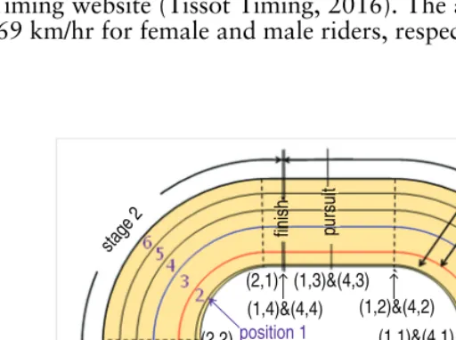
marks (the solid longitudinal lines shown in Figure 1) for each of the races were found. Times were determined to an accuracy of 1/50th second. Positions were or-dinally categorized and were also collected at each mark and each virtual mark as shown in Figure 1 (11 marks in total). The track is not flat but slopes upwards, linearly from the inside. The slope is greatest at the apex of the curves. Using the known three-dimensional geometry of the track and the information collected from video footage, riders’ average speeds over a stage were estimated; this is discussed further in Moffatt et al. (2014). The flying speeds of riders from the qualifying round were obtained from the Tissot Timing website (Tissot Timing, 2016). The average flying speeds were 63 km/hr and 69 km/hr for female and male riders, respectively (see Table 1).
stage 2
stage 3
measuring line
sprinter’s line stayer’s line
stages 1 and 4
200m line
finish pursuit
pursuit
100m line
(2,1)
(2,2) (2,3)
(3,1) (3,2) (3,3)(3,4)
(1,3)&(4,3)
(1,4)&(4,4) (1,2)&(4,2)
position 1 (1,1)&(4,1)
[image:11.635.138.394.347.538.2]The faster rider (rider with the faster flying speed) does not always win; in the dataset used to build the model, the faster rider won 71% of the time (see Table 1). The race is, therefore, highly tactical; broadly speaking, riders vie for track position in the first part of the race and sprint for the finish line in the second part. Riders typically cannot sustain an early sprint; flat out sprints from the start are rare and will be unsuccessful unless the trailing rider is taken by surprise or is much weaker. Therefore, throughout a race, a rider must make decisions about speed and position based upon an opponent’s speed and position, distance to the finish, and pre-race tactical plans. In each model (1–3), we assign the reference rider as the faster rider by ‘flying speed’, and the outcome is recorded from the point of view of this rider. For mod-elling, we divide the race into the following stages as shown in Figure 1. Stage 1 is the last 100 m of the first lap (600 m to 500 m to go). Moffatt et al. (2014) found race tactics not to be important prior to 600 m to go; therefore, this part of the race was not considered. At the end of stage 1, there are two laps (500 m) to go. Stage 2 is the next 50 m, stage 3 is the next 100 m and stage 4 is the final 100 m of the second lap (see Figure 1). Thus, four regressions are fitted at 500 m, 450 m, 350 m and 250 m to go. Tactically, the second lap is the crux of the race, and riders are committed to their actions as they enter the final lap: sprinting flat-out to hold the lead while staying inside the sprinter’s line or slipstreaming and overtaking around the final bend.
4.2 Model fitting procedure
Model 1 was fitted using the standard functions available in the R programming language (R Development Core Team, 2016). The fitting of Models 2 and 3 was im-plemented in MATLAB® (2007, Mathworks, Natick, Massachusetts), including the
variable selection procedure. The final set of covariates described in Tables 2 and 3, which includes first order interactions, was developed from the primary covariates (positions and average speeds). The final set of covariates relates to the average speed of the riders over stages, track position at the marks, changes of position and changes of lead (overtaking). In this example, over 30 covariates were considered at each stage. This made it impractical to use a variable selection technique which involved fitting all possible regressions and choosing between them using, for example, Akaike in-formation criterion or Bayesian inin-formation criterion (Dobson and Barnett, 2008). Instead, a procedure using bootstrap techniques in conjunction with forward step-wise was used (Sauerbrei and Schumacher, 1992). This involved generating bootstrap samples and fitting the regression to each bootstrap sample using forward stepwise to yield a bootstrap regression for each member of the bootstrap sample. Revealed covariates are selected for the final regression based on the number of times they appear in the bootstrap regressions. Although this procedure has been criticized for misselection (Austin, 2008), the broad view is that it selects covariates robustly.
As discussed in Section 3.3.1, for this application we assume that Zi−1 is
between the estimated score and the other covariates for the final model. Pearson product-moment correlation coefficient was calculated between the estimated score and the other covariates. No significant correlation (p-value less than 0.05) was found, indicating that this is also likely to be valid for the true score.
In order to directly compare Models 1 to 3, the same sets of covariates were used. These covariates were selected when applying the sequential model (Model 2) rather than the measurement error model (Model 3). This approach is likely to be more stringent because the sequential regression model is more optimistic about the size of effects, and this approach also had the advantage of reducing the computational burden (Moffatt, 2012).
4.3 Results
Tables 2 and 3 show how the interpretative complexity of the na¨ive sequential regression (Model 1) increases through the stages. The parameter estimates are generally more significant and the standard errors are generally larger for the na¨ive sequential model (Model 1). There are many more covariates in the na¨ive sequential models; therefore, there are not as many events (event being the outcome which occurred less often, i.e., win or lose in this case) per covariate term. Even at 450 m to go, there are only nine events per covariate term, reducing to five events per covariate term at 250 m to go. This suggests that the na¨ive sequential models in general are likely to be unstable/poorly estimated at later stages, particularly when there are many covariates in the models. Peduzzi et al. (1996) found in a simulated study that the variability in the parameter estimates becomes large and, hence, inaccurate when there are less than 10 events per covariate.
The sequential regression (Model 2) reduces this complexity; however, as discussed in Section 3, the sequential model assumes that the estimated score is measured without error, which is not true. When accounting for error in the score (Model 3) with a well-established measurement error method for our dataset, the estimated effect of the score at each stage is between 16% and 19% higher than when not accounting for error in the score (Model 2). This indicates that not accounting for the error in the score can lead to the estimate of the effect of the true unknown score being biased towards zero. The parameter estimates for most of the revealed covariates are similar for the sequential and sequential measurement error models. Therefore, the effect of the actions riders apply on win probability at each stage is similar for the sequential and sequential measurement error models. The key actions and race states that appear to influence race outcome at each stage are described in the next sub-section. However, the sequential model which underestimates the effect of the true unknown score, therefore, conversely overestimates the effects of revealed covariates. In this way, the sequential model places more importance on race actions and less on the ratio of flying speeds (the covariate that dominates the score) than the sequential measurement error model.
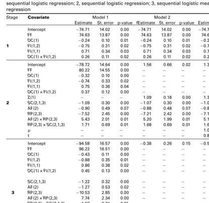
Table 2 Parameter estimates, standard errors andp-values for the three models at stages 1, 2 and 3: 1, na¨ive sequential logistic regression; 2, sequential logistic regression; 3, sequential logistic measurement error regression
Stage Covariate Model 1 Model 2 Model 3
Estimate St. error p-value fEstimate St. error p-value Estimate St. error p-value Intercept −74.71 14.02 0.00 −74.71 14.02 0.00 −74.71 14.02 0.00
FF 74.63 13.87 0.00 74.63 13.87 0.00 74.63 13.87 0.00
DC(1) −0.24 0.10 0.01 −0.24 0.10 0.01 −0.24 0.10 0.01
1 FI(1,2) −0.75 0.31 0.02 −0.75 0.31 0.02 −0.75 0.31 0.02
FI(1,1) 0.71 0.34 0.03 0.71 0.34 0.03 0.71 0.34 0.03
DC(1) ×FI(1,2) 0.26 0.11 0.02 0.26 0.11 0.02 0.26 0.11 0.02
Intercept −78.72 14.64 0.00 1.56 0.66 0.02 1.32 0.68 0.05
FF 80.22 14.55 0.00 − − − − − −
DC(1) −0.32 0.10 0.00 − − − − − −
FI(1,2) −0.74 0.33 0.02 − − − − − −
FI(1,1) 0.75 0.36 0.04 − − − − − −
DC(1) ×FI(1,2) 0.37 0.12 0.00 − − − − − −
Z(1) − − − 1.09 0.18 0.00 1.30 0.22 0.00
2 SC(2,1,3) −1.09 0.30 0.00 −1.07 0.30 0.00 −1.04 0.30 0.00
AF(2) −0.90 0.49 0.07 −0.88 0.48 0.07 −0.83 0.49 0.09
RP(2,3) −7.52 2.45 0.00 −7.21 2.42 0.00 −7.15 2.49 0.00
AF(2) ×RP(2,3) 5.43 2.01 0.01 5.20 1.99 0.01 5.16 2.04 0.01
RP(2,3) ×SC(2,1,3) 1.71 0.69 0.01 1.68 0.69 0.01 1.62 0.71 0.02
μ − − − − − − 1.07 0.05 −
t − − − − − − 0.85 0.04 −
Intercept −94.58 16.57 0.00 −0.38 0.26 0.15 −0.54 0.29 0.06
FF 96.22 16.51 0.00 − − − − − −
DC(1) −0.43 0.11 0.00 − − − − − −
FI(1,2) −0.88 0.35 0.01 − − − − − −
FI(1,1) 0.86 0.38 0.02 − − − − − −
DC(1) ×FI(1,2) 0.45 0.13 0.00 − − − − − −
SC(2,1,3) −1.22 0.32 0.00 − − − − − −
AF(2) −1.27 0.53 0.02 − − − − − −
3 RP(2,3) −10.53 2.85 0.00 − − − − − −
AF(2) ×RP(2,3) 7.74 2.34 0.00 − − − − − −
RP(2,3) ×SC(2,1,3) 1.93 0.74 0.01 − − − − − −
Z(2) − − − 1.21 0.17 0.00 1.40 0.20 0.00
SLI(3,3) 0.84 0.29 0.00 0.80 0.28 0.00 0.85 0.30 0.00
FI(3,1) −1.90 0.47 0.00 −1.86 0.46 0.00 −1.87 0.48 0.00
SI(3,1) −0.26 0.40 0.52 −0.28 0.39 0.47 −0.31 0.41 0.44
FI(3,1) ×SI(3,1) 2.50 0.67 0.00 2.43 0.65 0.00 2.44 0.67 0.00
μ − − − − − − 1.14 0.06 −
t − − − − − − 1.04 0.05 −
Note:See Table 4 for the definitions of the covariates. Parameter estimates with p-values greater than 0.05 were only retained in the model to conform with the hierarchical principle.
Table 3 Parameter estimates, standard errors andp-values for three models at stage 4: 1, na¨ive sequential logistic regression; 2, sequential logistic regression; 3, sequential logistic measurement error regression
Stage Covariate Model 1 Model 2 Model 3
Estimate St. error p-value Estimate St. error p-value Estimate St. error p-value
Intercept −94.12 17.68 0.00 0.38 0.21 0.07 0.24 0.22 0.28
FF 96.54 17.62 0.00 − − − − − −
DC(1) −0.48 0.12 0.00 − − − − − −
FI(1,2) −0.97 0.38 0.01 − − − − − −
FI(1,1) 1.09 0.41 0.01 − − − − − −
DC(1) ×FI(1,2) 0.51 0.14 0.00 − − − − − −
SC(2,1,3) −1.18 0.35 0.00 − − − − − −
AF(2) −1.61 0.59 0.01 − − − − − −
RP(2,3) −10.36 3.06 0.00 − − − − − −
AF(2) ×RP(2,3) 7.36 2.45 0.00 − − − − − −
RP(2,3) ×SC(2,1,3) 2.16 0.81 0.01 − − − − − −
4 SLI(3,3) 0.86 0.34 0.01 − − − − − −
FI(3,1) −1.83 0.51 0.00 − − − − − −
SI(3,1) −0.38 0.44 0.38 − − − − − −
FI(3,1) ×SI(3,1) 2.56 0.72 0.00 − − − − − −
Z(3) − − − 1.02 0.14 0.00 1.19 0.17 0.00
FLD(3,4) −1.07 0.42 0.01 −0.93 0.40 0.02 −0.92 0.41 0.02
DH(4,4) 0.00 0.05 0.92 −0.01 0.04 0.75 −0.02 0.04 0.63
UO(N,4)
UO(O,4) −2.31 0.81 0.00 −2.13 0.77 0.01 −1.85 0.72 0.01
UO(U,4) 0.03 0.66 0.97 −0.14 0.63 0.83 −0.16 0.72 0.83
DH(4,4) ×UO(N,4)
DH(4,4) ×UO(O,4) 1.60 0.63 0.01 1.60 0.63 0.01 1.43 0.67 0.03
DH(4,4) ×UO(U,4) 0.03 0.15 0.82 0.04 0.14 0.78 0.07 0.15 0.62
μ − − − − − − 1.30 0.07 −
t − − − − − − 1.35 0.06 −
Note:See Table 4 for the definitions of the covariates. Parameter estimates with p-values greater than 0.05 were only retained in the model to conform with the hierarchical principle.
Accounting for the error in the score also led to differences in the predicted win probabilities, which generally increase with the stage. At 450 m to go, for the majority of races, these differences are within the range −0.02 and 0.02, with 308 (87%) races being within this range (see Table 5). At 350 m to go and 250 m to go, 114 (32%) and 127 (36%) races have an absolute difference greater than 0.02, respectively (see Table 5). This illustrates that in a sequential approach, the effects of measurement errors propagate through stages.
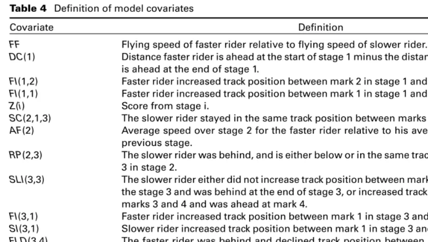
Table 4 Definition of model covariates
Covariate Definition
FF Flying speed of faster rider relative to flying speed of slower rider.
DC(1) Distance faster rider is ahead at the start of stage 1 minus the distance the faster rider is ahead at the end of stage 1.
FI(1,2) Faster rider increased track position between mark 2 in stage 1 and the end of stage 1.
FI(1,1) Faster rider increased track position between mark 1 in stage 1 and the end of stage 1.
Z(i) Score from stage i.
SC(2,1,3) The slower rider stayed in the same track position between marks 1 and 3 in stage 2.
AF(2) Average speed over stage 2 for the faster rider relative to his average speed in the previous stage.
RP(2,3) The slower rider was behind, and is either below or in the same track position at mark 3 in stage 2.
SLI(3,3) The slower rider either did not increase track position between marks 3 and the end of the stage 3 and was behind at the end of stage 3, or increased track position between marks 3 and 4 and was ahead at mark 4.
FI(3,1) Faster rider increased track position between mark 1 in stage 3 and the end of stage 3.
SI(3,1) Slower rider increased track position between mark 1 in stage 3 and the end of stage 3.
FLD(3,4) The faster rider was behind and declined track position between mark 3 in stage 4 and the end of stage 4.
DH(4,4) Distance the faster rider was ahead at mark 4, in stage 4.
UO(N,4) Neither rider over or undertook in stage 4.
UO(O,4) A rider overtook in stage 4.
UO(U,4) A rider undertook in stage 4.
Table 5 Number of races by the absolute difference in win probabilities for the faster rider at 450 m, 350 m and 250 m to go as predicted by the sequential and measurement error models
Model Difference in probability
≤0.01 0.01–0.02 0.02–0.03 0.03–0.04 0.04–0.05 0.05–0.1 >0.1
450 m to go 221 87 24 6 5 5 7
350 m to go 147 94 43 21 12 20 18
250 m to go 134 90 46 27 20 25 9
Note:At 450 m and 350 m to go 12 races and at 250 m to go 16 were excluded due to missing values.
[image:16.635.54.467.365.422.2]Table 6 The average difference between the probabilities predicted by the sequential (Model 2) and sequential measurement error (Model 3) models (sequential minus measurement error) by the estimated score and measurement error variance
Estimated Score Measurement error variance
Low (<0.05) Medium (0.05>=and<=0.15) High (>0.15)
Low (<0.5) 0.013(45) 0.004(46) −0.051(17)
Medium (0.5≥1.5) −0.004(55) −0.004(71) −0.005(16)
High (≥1.5) N/A −0.003(56) 0.02(49)
Note:The numbers in the brackets refers to the number of races.
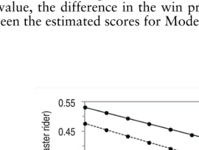
When the measurement error variance is low and the estimated score is extreme, the sequential measurement error model predicts a more extreme probability of winning for the faster rider, as there is more certainty in the estimated score. Tables 6 and 7 show the average difference predicted by the two models and Figure 2 shows an example of the effect a low measurement variance has on the predicted win probabilities for one race. The exception is when the estimated score for Model 3 is less extreme in comparison to the estimated score for Model 2. Then, the opposite becomes true in that the measurement error model predicts the less extreme probability. When the estimated score or measurement error variance is close to the median value (over all races), the win probabilities are similar at 450 m to go. At both 350 m and 250 m to go, when the estimated score for Model 3 is close to the median value, the difference in the win probabilities mostly depends on the difference between the estimated scores for Models 2 and 3.
Win probability (faster rider)
0.55
0.45
0.35
0.25
0.15
AF(2): Average speed of the faster rider
overstage 2 compared to stage 1
0.95 1.15 1.35 1.55 1.75
Figure 2 Win probability for the faster rider at 450 m to go (end of stage 2) as a function ofAF(2), when
SC(2,1,3) = 1 andRP(2,3) = 0 (see Table 4 for covariate definitions) for three cases with a low scoreZ(1), (–x–) =
[image:17.635.160.365.403.557.2]0.6
0.55
0.5
0.45 0.65 0.7 0.75
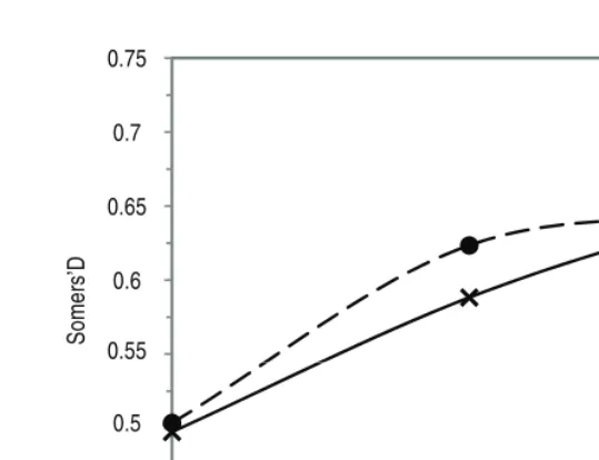
Somers’D
250 300
350 400
450
[image:19.635.130.400.88.295.2]Distance (m) to go
Figure 3 The association between observed and predicted responses at each stage for the sequential model (–•–) and the measurement error model (–x–) as measured by Somers’ D (adjusted using Efron’s 0.682 estimator).
The fit of both Models 2 and 3 were compared by calculating the Somers’ D value, which is a measure of association between the observed and predicted responses. No extra data was available to test how well the models fit on a different dataset. Instead, the Somers’ D value was calculated on the same dataset used to build the model, but this value was adjusted using Efron’s 0.682 estimator (Efron, 1983), which is used to adjust for the over-optimism in a Somers’ D value which is calculated based on the dataset used to fit the model. The Somers’ D value was similar for both the sequential and sequential measurement error models at all stages, with some evidence of the sequential model performing better at 350 m to go (see Figure 3). However, because large differences in the probabilities predicted between Models 2 and 3 were found for only a few races, the differences between the Somers’ D values will also be small.
4.4 Summary of tactical implications
8 10 12
% of races
2
0 4 6
250 300
350 400
450 500
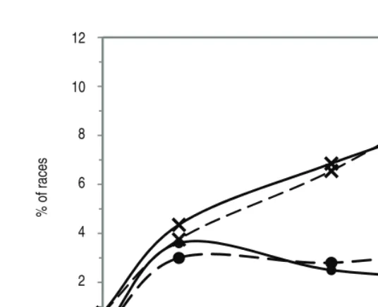
[image:20.635.127.395.87.305.2]Distance to go (m)
Figure 4 Percentage of races accounted for by race states and actions: (–x–) applied up to and including the end of the current race stage, (–•–) during the current stage for the sequential (– – –) and sequential
measurement error models ( ).
(71%). This gives the proportion of races for which race states and actions applied before the end of each stage are influential. This is similar for both models, only 1% at 500 m to go rising to 9% at 250 m to go for the sequential model and slightly lower (8%) at 250 m to go for the measurement error model. Figure 4 also shows the proportion of races which can be accounted for by the actions and states applied during each stage (the percentage of race outcomes correctly predicted over and above that predicted by assuming that the faster rider wins at the current stage minus that at the previous stage), which remains approximately constant between 450 m and 250 m to go at around 3% for both models. Overall, the similar performance is not surprising considering that for the majority of races, the predicted win probabilities are similar for the two approaches.
As discussed in the previous section, the parameter estimates for both models are similar and so are the key actions and race states that appear to influence race outcome. From the parameters estimates which are displayed in Tables 2 and 3, the key actions and race states that appear to influence race outcome are identified for each stage.
save energy for later in the race. A faster rider who is following should reduce the distance behind if following.
In stage 2, the slower rider can take advantage, if the opponent is not accelerating, by being behind and either in the same track position or lower than the faster rider by the end of the stage. The slower rider should also change track position between marks 1 and 2 in stage 2. Changing track position may allow the rider to save energy where the track gradient is high.
In stage 3, the faster rider has a very low chance of winning if he/she increases track position between mark 2 and the end of stage 3 when the opponent does not increase track position. This implies the faster rider has wasted energy by increasing track position and, hence, loses an advantage at later stages in the race.
In stage 4, both riders should overtake if behind; the faster rider should also be far ahead (>2 m). It is better to overtake than undertake or already be leading the race at the beginning of this stage. A faster rider who is behind and does not over take or under take considerably reduces his/her chances of winning by decreasing track position during this stage (see Table 2;FLD(4) = 1), as the rider may have been unsuccessful in overtaking during this stage, and so overtaking during the remainder of the race will be more difficult to achieve.
5 Discussion and conclusion
A new approach is presented for analyzing the relationship between the outcome of a process with several stages and covariates that are revealed at each stage when the number of influential covariates is large. The approach extends the sequential model of Elisheva et al. (2000) by accounting for the measurement error in the estimated score. The approach is applied to the sprint event in track cycling with the aim of explaining race outcome and the following is found:
1. The score allows stable models to be created while capturing information from previous stages. Fewer terms in a sequential approach (in comparison to the na¨ive approach) also mean that the models are easier to interpret.
2. However, the score is measured with an error. A new approach is developed to incorporate for this error and we show for our application that not accounting for measurement error in the score leads to the estimated effect of the score being biased. For other terms, the bias is small, except for terms where the corresponding states or actions occurred infrequently in the dataset. The sequential model places more importance on race actions and less on the ratio of flying speeds (the covariate that dominates the score) than the sequential measurement error model.
via conversion to a score leads to an even more extreme probability. For some races, the probabilities predicted by the sequential model are unrealistically high or low, which are compounded at later stages. The sequential model predicts high chances of outcomes at 450 and 350 m to go for some races, but for this event it is highly unlikely that the outcome of the race has been decided at this stage. This illustrates that the measurement errors propagate through the stages in a sequential approach.
4. The measurement error technique adjusts the win probabilities (compared to the sequential approach) depending on the magnitude of the measurement error. The measurement error model predicts more extreme win probabilities when the measurement error variance is low and less extreme win probabilities when the measurement error variance is high. At stages 3 and 4, this effect also depends on the difference between the sequential and estimated scores, with the measurement error model predicting more extreme probabilities if the estimated score is more extreme and vice versa.
It is assumed that the true score is not correlated with the other observed covariates revealed in the current stage. This assumption is tested and shown to be valid for the application we described in Section 4. However, this may not be the case for a different application. Future work could involve adjusting the model to allow for such correlations. The approach could also be readily extended to incorporate variable selection techniques when little prior information is available about which covariates are influential on outcome.
Overall, we would suggest that it is essential to use measurement error techniques in a sequential approach to avoid bias in the estimation of the parameter for the score and, hence, to avoid misleading conclusions being drawn when determining the effects of covariates on outcome, especially when considering the relative importance of previous and current actions and states. These conclusions are applicable to the statistical analysis of sequential processes more generally outside of the sports example presented in this article, including, for example, medical intervention where extreme predicted probabilities could lead to the wrong decision being made about the most appropriate treatment. The real benefit of this approach will vary with application and may be assessed by preforming simulations.
Acknowledgements
References
Austin PC (2008) Bootstrap model selection had similar performance for selecting authentic and noise variables compared to backward variable elimination: A simulation study. Journal of Clinical Epidemiology,61, 1009– 1017.
Carroll RJ, Ruppert D, Stefanski LA and
Crainiceanu CM (2006) Measurement
Error in Nonlinear Models: A Modern Perspective, 2nd edition. Boca Raton, FL: CRC Press.
Collett D (2002)Modelling Binary Data, 2nd
edi-tion. Boca Raton, FL: CRC Press.
Dobson AJ and Barnett AC (2008)An
Introduc-tion to Generalized Linear Models, 3rd
edi-tion. Boca Raton, FL: CRC Press.
Efron B (1983) Estimating the error rate of a prediction rule: Improvement on
cross-validation. Journal of the American
Statis-tical Association,78, 316–331.
Efron B and Tibshirani RJ (1993)An Introduction
to the Bootstrap. New York and London: CRC Press.
Elisheva S, Noya G, Yana Z-G, Dalit B and Benjamin M (2000) Sequential logistic mod-els for 30 days mortality after CABG: Pre-operative, intra-operative and post-operative experience—The Israeli CABG
study (ISCAB). European Journal of
Epi-demiology,16, 543–555.
Guo Y and Little RJ (2011) Regression analy-sis with covariates that have heteroscedastic
measurement error. Statistics in Medicine,
30, 2278–2294.
Higdon R and Schafer DW (2001) Maxi-mum likelihood computations for
regres-sion with measurement error.
Computa-tional Statistics & Data Analysis, 35, 283–299.
Hildebrand FB (1974) Introduction to
Numeri-cal Analysis, 2nd edition. New York and London: McGraw-Hill.
Hill SE, van Wermeskerken GK, Lardenoye J-WH, Phillips-Bute, B, Smith PK, Reves JG and Newman MF (2000) Intraoperative phys-iologic variables and outcome in cardiac
surgery: Part i. In-hospital mortality. The
Annals of Thoracic Surgery, 69, 1070– 1075.
MATLAB (2007). The MathWorks Inc., Natick, Massachusetts.
McCullagh P and Nelder JA (1989)Generalized
Linear Models, 2nd edition. Boca Raton, FL: CRC Press.
Moffatt JL (2012) Sequential regression
techniques with application to the in-dividual sprint in track cycling. PhD thesis, Salford Business School, University of Salford, Salford, UK.
Moffatt JL, Scarf P, McHale IG, Passfield L and Kui Z (2014) To lead or not to lead:
Anal-ysis of the sprint in track cycling. Journal
of Quantitative Analysis in Sports,10, 161– 172.
Peduzzi P, Concato J, Kemper E, Holford TR, and Feinstein AR (1996) A simulation study of the number of events per variable in logistic
regression analysis.Journal of Clinical
Epi-demiology,49, 1373–1379.
R Development Core Team (2016)R: A Language
and Environment for Statistical
Comput-ing. Vienna, Austria: R Foundation for
Statistical Computing. URL
http://www.R-project.org. (Accessed on 21 June
2016).
Rabe-Hesketh S, Pickles A and Skrondal A (2003) Correcting for covariate measurement error in logistic regression using nonparametric
maximum likelihood estimation.Statistical
Modelling,3, 215–232.
Rosner B, Spiegelman D and Willett W (1990) Correction of logistic regression rela-tive risk estimates and confidence inter-vals for measurement error: The case of multiple covariates measured with error. American Journal of Epidemiology, 132, 734–745.
Sauerbrei W and Schumacher M (1992) A boot-strap resampling procedure for model build-ing: Application to the cox regression
model. Statistics in Medicine, 11, 2093–
2109.
Seber GA and Lee AJ (2012)Linear Regression
Thoresen M and Laake P (2000) A simula-tion study of measurement error correcsimula-tion
methods in logistic regression. Biometrics,
56, 868–872.
Tissot Timing (2016) Track cycling results. URL http://www.tissottiming.com/
UCI (2016) Track cycling information. URL http://www.uci.ch/
Van Wermeskerken GK, Lardenoye J-WH, Hill SE, Grocott HP, Phillips-Bute B, Smith PK, Reves JG, and Newman MF (2000) In-traoperative physiologic variables and out-come in cardiac surgery: Part ii. Neurologic
outcome.The Annals of Thoracic Surgery,
69, 1077–1083.
Vittinghoff E and McCulloch CE (2007) Relaxing the rule of ten events per variable in
logis-tic and cox regression.American Journal of
Epidemiology,165, 710–718.
Welsby IJ, Bennett-Guerrero E, Atwell D, White WD, Newman MF, Smith PK and Mythen MG (2002) The association of complica-tion type with mortality and prolonged stay after cardiac surgery with cardiopulmonary
bypass.Anesthesia & Analgesia,94, 1072–