A Wavelet-ARIMA Model for Drought Forecasting using SPI Data

(1)

International Journal of Emerging Technology and Advanced Engineering

Website: www.ijetae.com (ISSN 2250-2459, ISO 9001:2008 Certified Journal, Volume 9, Issue 10, October 2019)

86

A Wavelet-ARIMA Model for Drought Forecasting using SPI

Data

Mohammed Salisu Alfa

1

, Ani Bin Shabri

2

, Muhammad Akram Shaari

3

1,2

Department of Mathematical Sciences, Faculty of Science, Universiti Teknologi Malaysia (UTM) 81300 Johor, Malaysia 3_{School of Computing, Faculty of Engineering, Universiti Teknologi Malaysia (UTM) 81300 Johor, Malaysia}

Abstract— This paper is on the Wavelet-Auto-Regressive

Integrated Moving Average (W-ARIMA) model to see to the ability of the propose model over an ARIMA model. The new model was developed by combining the ARIMA model with the Discrete Wavelet Transform (DWT) using the Standardized Precipitation Index (SPI) drought data for forecasting. The models were used on four SPI data sets which includes SPI3, SPI6, SPI9 and SPI12 data series. To assess the potential of the new model for drought forecasting. to achieve this, a 624 month of SPI data from January 1956 to December 2008 was used and were divided into two parts (80% for training and 20% for testing). The result of the W-ARIMA models for forecasting were compared with that of the traditional ARIMA model using the Root Mean Square Error (RMSE), Mean Average Error (MAE) and coefficient of correlation (R) as the performance statistical error measures used. The results of the proposed model (W-ARIMA) and that of the ARIMA model showed very clearly that the propose method achieved the best drought forecasting performance in terms of accuracy for each of the SPI data series. This indicates that W-ARIMA model outperform the traditional ARIMA model in SPI drought forecasting. Similarly, SPI12 data showed that it has the minimum error among all the SPI data series used in the work.

Keywords—ARIMA, Wavelet, SPI, DWT, Drought

Forecasting.

I. INTRODUCTION

TTo ease the comparison between ARIMA and Wavelet–ARIMA model, four SPI drought data series are used for forecasting. Drought forecasting all over world is a subject which has been carried out by different researchers to apply different models to achieve their goals. Drought forecasting with SPI data is very important in management of water resources and planning for all creatures. Referring to the work of [1], time series forecasting have commonly been used in a wide range of scientific applications that includes meteorology and hydrology. Drought is described by [2] as one of natural phenomenon involving climate which is the first natural disaster in the world over which affects places and inflicting significant damages to both human beings and the environment in which they live.

The opinion of [3], described drought as a normal feature of climate that occur which is due to rainfall that is below average in a place that leads to shortage of water, loss in economic activity and unexpected reduction in precipitation over time which is one of the most harmful natural disasters that affects human beings.

In the current and various studies therefore, time series forecasting has commonly been used. [4], sees time series forecasting as one of the important research areas in analyzing the hydrological time series. On the other hand, [5] is of the view that time series forecasting is an act of predicting the future by understanding the past. Time series forecasting has become an important approach to drought forecasting whose application is widely used [6]. In the view of [7], forecasting techniques which have been developed with the evaluation performance in other to forecast future values of a time series is one of the areas in time series analysis. The principal aim of time series forecasting is to forecast future events based on known past data or an event.

SPI data series has a wide application for the description of drought in different period. SPI data series is therefore expected to serve as a data input in the ARIMA model to be measured using only precipitation SPI data which were applied for drought analysis. ARIMA model is a Box Jenkins methodology named after the original authors, Box and Jenkins, 1969 which seeks to transform any time series data to be stationary after which the data is then applied for forecasting using the past univariate time series process for future forecast with some selection and diagnostic tools. ARIMA model is very popular due to its flexibility in representing several varieties of time series with the associated Box-Jenkins methodology [8] and [9].

Also, in a separate analysis, ARIMA model was combined with wavelet and therefore, the discrete wavelet transforms (DWT) was used because of its simplicity and shorter time for computation purposes which serves as an alternative in forecasting applications. The wavelet-ARIMA model can achieve a better forecasting accuracy

(2)

International Journal of Emerging Technology and Advanced Engineering

87

The existing forecasting ARIMA model was improved upon in the forecast of climate time series by using wavelet transform (Rahman and Hasan 2014).

The wavelet transformation has the basic objective of being able to do the analysis of the time series data involving time and frequency domain by decomposing the original time series in different frequency bands because wavelets are tools which are important in time series forecasting. with the use of wavelet functions. The wavelet transforms are mathematical functions which can be used for the analysis of time series with non-stationarities. This wavelet technique allows the use of long-time intervals for low frequency information and short time intervals for high frequency information that can reveal aspects of data like trends. Another merit of wavelet analysis is the flexibility of the choice of the mother wavelet in accordance with the characteristics of the time series that is investigated Wavelet transform also has the advantage of allowing the study of various independent treatments on distinct time scales.

II. METHODOLOGY

Both ARIMA model and Wavelet have been found to be very effective in the areas of drought forecasting generally and has been applied in many fields such as drought, flooding, river flow and streamflow. This study is motivated by the application of SPI data to obtain the best ARIMA model and to combine it with the wavelet to get W-ARIMA model for each of the SPI data series.

The main objective of this study is to combine wavelet with the ARIMA model for the drought forecasting using SPI data series and to compare the traditional ARIMA model with DWT method to obtain the proposed model (W-ARIMA model)

A Auto-Regressive Integrated Moving Average (ARIMA) Model

One of the most widely used time series models is the ARIMA model whose popularity is due to its statistical properties as well as the Box-Jenkins methodology in the building process [9]. With ARIMA model, complex patterns in the data which can also be used to generate forecast (Box and Jenkins, 1976). In responding to time series as a linear combination of its past values, ARIMA model could predict a value or values [14].

Based on the approach of Box and Jenkins, ARIMA models for the SPI time series were developed on three steps: model identification, parameter estimation and diagnostic checking.

The details on the development of ARIMA models for SPI time series can be found in the works of [15].

ARMA time series which is made stationary due to differencing process is referred to as ARIMA model. ARIMA model is made up of three parameters namely P (order of autoregressive model), d (order of differencing) and q (order of moving average model). ARIMA models are one of the most important forecasting models that have been successfully applied in modeling and forecasting, [6]. If AR, I, or MA are dropped in description the model. E.g. ARIMA (1, 0, 0) is AR (1), ARIMA (0, 1, 0) is 1(1) and ARIMA (0, 0, 1) is MA (1).

If AR, I, or MA are dropped in describing the model. E.g. ARIMA (1, 0, 0) is AR (1), ARIMA (0, 1, 0) is 1(1) and ARIMA (0, 0, 1) is MA (1).

For a non-seasonal ARIMA models, the equation is given by:

1 1 1

1 1

...

1 1

...

t t p t p t q t q t

X

 

C



X

_

 



X

_





e

_

 



e

_





(1)

Where: -

1 t

X

is the differenced series (It may have been differenced more than one time).

The “predictors” included both lagged values of Xt_and

lagged errors. This is referred to as ARIMA (p, d, q) model in which P = order of the autoregressive part, d = degree of first differencing involved, q = order of moving average

part,



,



are polynomials of order p and q



1

...





1 



1

...



d

P q

P

X

t

C

q

e

t

 



 



 



  

 

(2)

First term referred to AR(p), Second term referred to d = differencing, RHS part referred to MA(q)

Selecting the appropriate values for p, d, and q can be difficult, hence, relevant software can be used.

For a seasonal series ARIMA models can model a wide range of seasonal data. It is formed by including additional seasonal terms in the ARIMA models like,

ARIMA (p, d, q) (P, D, Q) m which implies

(Non-seasonal part of the model) (Seasonal part of the model) and m is the number of periods per season. The seasonal part of the model is made up of terms that are very similar to the non-seasonal components of the model, however, they involve backshifts of the seasonal period. For instance, An ARIMA (1, 1, 1) (1, 1, 1)4 model (without a constant

(3)

International Journal of Emerging Technology and Advanced Engineering

88 





4



 

4







4



1 1 1 1

1

yt et

 



 



 



(3)

From the LHS,

First term represents Non-seasonal AR (1); Second term represents Seasonal AR (1); Third term represent Non-seasonal difference; Fourth term represents Seasonal difference. Then from the RHS, first term represents Non -seasonal MA (1); Second term represents Seasonal MA (1) It should be noted that the additional seasonal terms are simply multiplied by the non-seasonal terms.

Differencing is applied to time series data to make it stationary (which is a time series property which does not depend on the time at which the data is observed). [16] and [17] applied ARIMA model in drought forecasting.

B Wavelet Analysis

A wavelet is a mathematical function which is used in digital signal processing and image compression. Wavelet analysis is becoming a well-known tool because of its ability to show information within the signal in both the time and scale (i.e. frequency) domains [18]. Wavelet is a mathematical procedure that involves the transformation of the original signal (most especially in the time domain) into a different domain in processing and in the analysis [19].

[2], in his study of hybrid wavelet and adaptive neuro-fuzzy inference system for drought forecasting stated that wavelet analysis is one of the most powerful tools to study time series. In another study, [20], described wavelet analysis as a multi-decomposition analysis that provide information for time and frequency domains and provide useful decompositions of the original time series for the wavelet–transformed data to improve the power of a forecasting model. Wavelet is a tool in time series forecasting whose importance is applied by many researchers. One of the basic objectives of wavelet transforms is to analyze the time series data. Wavelet transform can be categorized into continuous wavelet transform (CWT) and discrete wavelet transform (DWT). The former is not always used in forecasting because of its complex computational ability and the time needed for it [21]. In place of its DWT is mostly used in applications of forecasting to make numeric solutions simpler. Therefore, it requires less time for computation which is simple to apply. DWT is given by the formula:

 

0 0

,

0 0

1

m

m n _m m

t

n s

t

s











_





_





₍₄₎

Where



 

t

is the mother wavelet, m and n are integers that control the scale and time respectively. The

most common selections for the parameters

s

0_{=2 and}

0



_{=1. The Mallat’s theory has the original discrete time} series x(t) can be decomposed into a series of linearity independent approximation and detail signals by using the inverse DWT, which is given by Mallat, (1989) as





1

2

2 , 1 0

( )

2

M m

m

M _m

m n m t

x t

T

W



t n

 

 





 



(5)

Where





 

1

2 ,

1

2

2 m

N m m n

m

W



t n x t

 

 







is the wavelet coefficient for the discrete wavelet at scale s=2m and



=2m n

In the analysis, DWT is mostly preferred in the forecasting problems due to its simplicity and the ability to compute within a short period of time. Many researchers have undertaken studies in the field of water resources and hydrology using wavelet transforms which are based on data pre-processing. As pre-processing tool, wavelet transforms provide useful decomposition of the original time series so that the pre-processed data can improve the ability of a forecasting model by capturing the information based on different resolution levels [22]. Wavelet transform (WT) analysis have become an ideal tool for the study of a measured non-stationary times series through the hydrological process. The DWT requires less time for computation and simple to implement. DWT scales and positions are usually based on powers of two (dyadic scales and positions). This is achieved by modifying the wavelet representation. To [23], the DWT operates two sets of functions: high-pass and low-pass filters. DWT is the best known tool for data analysis whose contribution to model hydrological resources can be seen in the last few years [24].

(4)

International Journal of Emerging Technology and Advanced Engineering

89

In W-ARIMA, the original drought SPI data series was decomposed into several sub time series components which serve as input to ARIMA in other to improve the accuracy of the model. To obtain a number of decomposition level, the following formula by [25] is applied





int log( )

L



N

(6)

Where L is the decomposition level and N is the number of the SPI data series. In the formula, the original SPI

drought data series is decomposed into

L

components

from A to

D

L1 (A1, D1, D2. . ., L 1

D

_

) which stands for different frequency components of the original data. In this paper, the number of decomposition levels, N, is equal to 5. Instead of using the D’s component separately, as input model, we employ added suitable D’s component which is more useful and capable of increasing the forecast performances of the mode

The structure in fig.1 explains the development of proposed W-ARIMA model in which each wavelet is used to forecast the ARIMA model. This begins when SPI data series were pre-processed using DWT and values A, D1, D2, D3…D5 used as input to forecast each wavelet with ARIMA. This sub-series are summed and used as inputs to the original data to obtain the final forecasts using RMSE, MAE and R as the chosen performance measures.

C Wavelet-ARIMA (W-ARIMA) model results

The wavelet is combined with ARIMA model to form W-ARIMA model to form W-ARIMA. This is to improve the ability of ARIMA model for drought forecasting. The original SPI data series was decomposed into several data series components which were input to ARIMA to improve the accuracy of the model. For this, the original SPI drought data series is decomposed into five levels (A, D1,

D2, D3, D4, D5) using the given formula





int log( )

L



N

). The components of DWT are chosen as input to ARIMA model to improve the forecasting performance of the two models put together. The choice of these components of DWT is also to allow ARIMA model to determine the features of the SPI data series which produces a better estimation.

The forecasting ability of ARIMA model was improved upon by the application of Wavelet analysis with respect to all the SPI as shown on table 3. It also improved the forecasting performance measures. The significance of applying the DWT in the view of [25] is to smooth the analysis of SPI data obtained after the wavelet decomposition. Wavelet transform decomposes the SPI data into different number of component series to minimize the error criterion.

The wavelet transform was proposed to address some of the limitations which Fourier transform could not tackle using mother wavelets (basic functions) which are translated to give a good time resolution for the high-frequency events. To conduct wavelet analysis, one of the instruments used in determining the performance of the model in the wavelet domain is the choice of the optimal number of decomposition levels using [26] formula to choose the number of decomposition levels.

III. RESULTS AND DISCUSSIONS

(5)

International Journal of Emerging Technology and Advanced Engineering

90

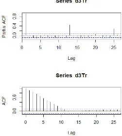
The selection of parameters for the ARIMA models are based on the PACF and ACF of the time series.as soon as significant lags were obtained from PACF and ACF, ARIMA models with different combinations were then developed and the model with the lowest RMSE and MAE and highest R were selected as contained on tables 1 and 2 was selected. Fig.3 shows the PACF and ACF plots.

Table1is made up of all the detail ARIMA model results using forecasting accuracy of MSE and MAE as the performance evaluation criterium which explains the detail results involving all the SPI data series. The results showed that SPI3 is a non-seasonal data while the rest three are seasonal data. The table also explains the detail result of each SPI data series.

(i)Fitted to the data, many diagnostic checks were carried out and if the models fit well, the residuals are expected to be uncorrelated wit constant variance, however, in the development of model this is usually assumed that the errors are normally distributed and for this, the residuals are expected to be normally distributed.

Figure 3 Showing the graphs of Standardized ACF and P-values of Residuals for all SPI data

Figure 1: Showing Time series plots of the SPI data sets

Figure2 indicates all the 624 data sets for each of the SPI data used for the study.

(ii) Model identification: - this involves the selection of model parameter (p, d, q) from the PACF and ACF plots

Figure 2 Showing the PACF and ACF graphs of SPI data Series

Fig.3 indicates all the plots of PACF and ACF where models are identified for seasonality and SPI3 exhibits non-seasonality, other SPI data like SPI6, SPI9 and SPI12 are seasonal, hence, seasonal ARIMA model was carried out in the analysis. The orders of p, d, q is required to determine the best model based on PACF and ACF observed values and after careful observation of the plots of graphs. SPI3 which exhibits non-seasonal from the plot shows a possible ARIMA (p, d, q) model with p = 3 and q = 1, the finally selected model after evaluation, was ARIMA (3, 0, 1) which was chosen. The residual ACF and PACF which has the best model is shown in fig.3. the ACF and PACF both lie within confidence limits.

[image:5.612.323.574.143.423.2] [image:5.612.54.276.414.525.2]

(6)

International Journal of Emerging Technology and Advanced Engineering

91

Since the models have been fitted to the data, many

diagnostic checks were carried out and if the models fit well, the residuals are expected to be uncorrelated wit constant variance, however, in the development of model this is usually assumed that the errors are normally distributed and for this, the residuals are expected to be normally distributed.

Figure 3 Showing the graphs of Standardized ACF and P-values of Residuals for all SPI data.

Standard checks for ARIMA is to compute the PACF and ACF of the residuals. Since the residuals are normally distributed, they lie on a straight upward sloping line. In evaluating the proposed model, the ARIMA involving time series was used to model SPI3, PI6, SPI9 AND SPI12 time series.

Table 1

Showing the Selected Best ARIMA Models

Training Testing

Data RMSE MAE R RMSE MAE R Spi3 Spi6 Spi9 Spi12 0.65539 0.42623 0.41937 0.36986 0.51548 0.33498 0.33133 0.29168 0.75463 0.90025 0.90250 0.92317 0.57406 0.40859 0.37645 0.36279 0.44702 0.31178 0.29047 0.27487 0.82073 0.91829 0.92970 0.93609

[image:6.612.64.498.249.499.2]

Table 1 above indicates the selected best ARIMA models obtained from the series of ACF and PACF and according to the performances of the standardized ACF and p-values in the various plots as indicated int the figures above.

Table 2

Showing the W-ARIMA Models obtained from the various wavelets

Training Testing

Data RMSE MAE R RMSE MAE R

Spi3 Spi6 Spi9 Spi12 0.31351 0.21244 0.20529 0.17463 0.23092 0.15699 0.14339 0.12240 0.95019 0.97619 0.97759 0.98342 0.29622 0.20112 0.16473 0.17544 0.22619 0.15835 0.12807 0.13438 0.95410 0.98035 0.98663 0.98501

[image:6.612.296.591.529.699.2]

Table 2 above indicates the W-ARIMA models obtained from the various wavelets.

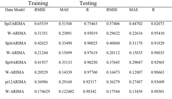
Figure 3

Showing the Comparison of ARIMA and W-ARIMA Models

Training Testing

Data Model RMSE MAE R RMSE MAE R

(7)

International Journal of Emerging Technology and Advanced Engineering

92

The table 3 above describes the various results of the analysis of training and testing carried out for all the SPI data series used. The results are the summary of the selected from the six inputs considered (inputs 2, 4, 6, 8, 10 and 12). For each model, the inputs with the least error (RMSE and MAE) and the highest coefficient of correlation (R) were selected for the purpose of comparison. In each of the SPI data, the W-ARIMA model recorded the least RMSE and MAE indicating that it is better than the ARIMA model in drought forecasting. The results indicate that Spi12 data has the smallest error in both ARIMA and W-ARIMA when compared with the other three data sets. This leads to the selection of W-ARIMA model as the best and being proposed as the appropriate model for drought forecasting

IV. FORECAST EVALUATION METHODS

The criteria in judging the best model are how relatively small the models are in both the training and testing of the data series. This is needed to be able to quantify the amount by which the estimator differs from the true (original) value. That is why the measures with smallest values are usually selected as the best model.

Evaluation of the performance of each model was based on the Mean Square Error (MSE) and Mean Absolute Error (MAE) for both training and testing which is used for this study. All these performance evaluation are widely used in obtaining the results of time series forecasting [27]. These are stated below:

1

n

_ˆ

i i

i

RMSE

y

n







(7)









n t t t

y

n

MAE

1

|

ˆ

|

1

(8) 2 / 1 1 2 2 / 1 1 2 1

)

ˆ

(

)

(

)

ˆ

)(

(

































   n t t t n t t t n t t t t t

y

R

(9)

Where

X

ˆ

_i is the predicted value,

X

_iis the actual value

at time i, and n is the number of Predictions

V. CONCLUSION

In this study, wavelet transforms and ARIMA model were combined to develop a hybrid model for forecasting the SPI drought data. Firstly, ARIMA model was used to model the SPI data series without prepossessing the data. Secondly, the proposed hybrid model was obtained by combining ARIMA with wavelet transforms was used to capture the multi-scale features of the SPI data series used to decompose the data. In the study also, the new SPI data series obtained with the addition of effective wavelet components which was used as output to the ARIMA model used to forecast the SPI drought. The performance evaluation of the proposed W-ARIMA model which was based on MSE and MAE was then compared with ARIMA model which indicated a great improvement in SPI drought modeling and produced a better forecast result than the individual ARIMA model. we then concluded that the forecasting capability of W-ARIMA was found to be improved upon when the wavelet transformation technique was used for data preprocessing. The decomposed periodic components obtained from DWT technique were found to be very effective in getting accurate forecasts when it was used as inputs in ARIMA model. the results for the forecasts is an indication that the W-ARIMA model provides an alternative forecasting model to other models and serves as a potential hope as a new method to be used in SPI drought forecasting.

REFERENCES

[1] V. Shah, Ravi, Bharadiya, Nitin, Manekar, “Drought index computation using standardzed precipitation index (spi) method for surat district Gujarat,” J. Hydrol., vol. 391, no. 1–2, pp. 202–216, 2010.

[2] A. Shabri, “A hybrid wavelet analysis and adaptive neuro-fuzzy inference system for drought forecasting,” Appl. Math. Sci., vol. 8, no. 139, pp. 6909–6918, 2014.

[3] Dalwadi, “The Wavelet Tutorial,” Internet Resour. httpengineering rowan edu polikarWAVELETSWTtutorial html, pp. 1–67, 2016. [4] L. I. Shijin, “Procedia Engineering,” Appl. Math. Sci., 2012. [5] T. Raicharoen and C. Lursinsap, “A divide-and-conquer approach to

the pairwise opposite class-nearest neighbor (POC-NN) algorithm,” Pattern Recognit. Lett., vol. 26, no. 10, pp. 1554–1567, 2005. [6] Zhang, “A review of drought concepts,” 2013.

[7] C. Cordeiro and M. Neves, “Forecasting time series with Boot. EXPOS procedure,” Revstat, vol. 7, no. 2, pp. 135–149, 2009. [8] C. Hamzacebi, “Improving artificial neural networks’ performance

in sseasonal time series forecasting,” Prentice Hall, vol. 178, no. 23. pp. 4550–4559, 2008.

(8)

International Journal of Emerging Technology and Advanced Engineering

93

[10] W. Wei et al., “Application of a combined model with autoregressive integrated moving average (arima) and generalized regression neural network (grnn) in forecasting hepatitis incidence in heng county, China,” PLoS One, vol. 11, no. 6, pp. 1–13, 2016. [11] G. Kirschgässner and J. Wolters, Introduction to Modern Time

Series Analysis. 2007.

[12] E. Szolgayová, J. Arlt, G. Blöschl, and J. Szolgay, “Wavelet based deseasonalization for modelling and forecasting of daily discharge series considering long range dependence,” pp. 24–32, 2014. [13] P. Udom and N. Phumchusri, “A comparison study between time

series model and ARIMA model for sales forecasting of distributor in plastic industry,” vol. 4, no. 2, pp. 32–38, 2014.

[14] X. Zhang, Y. Peng, C. Zhang, and B. Wang, “Are hybrid models integrated with data preprocessing techniques suitable for monthly streamflow forecasting ? Some experiment evidences,” J. Hydrol., vol. 530, pp. 137–152, 2015.

[15] A. K. Mishra and V. P. Singh, “Drought modeling - A review,” J. Hydrol., vol. 403, no. 1–2, pp. 157–175, 2011.

[16] P. Han, P. Wang, M. Tian, S. Zhang, and J. Liu, “Application of the ARIMA Models in Drought Forecasting Using the Standardized Precipitation Index,” 2012.

[17] P. Han et al., “Application of the ARIMA Models in Drought Forecasting Using the Standardized Precipitation Index To cite this version : HAL Id : hal-01348118 Application of the ARIMA Models in Drought Forecasting Using the Standardized Precipitation Index,” 2016.

[18] V. Nourani, M. T. Alami, and F. D. Vousoughi, “Wavelet-entropy data pre-processing approach for ANN-based groundwater level modeling,” J. Hydrol., vol. 524, pp. 255–269, 2015.

[19] B. Dong, Y. Mao, I. D. Dinov, Z. Tu, and Y. Shi, “Wavelet-Based Representation of Biological Shapes Wavelet-Based Representation of Biological,” no. June 2014, 2009.

[20] A. Shabri and R. Samsudin, “Fishery Landing Forecasting Using Wavelet-Based Autoregressive Integrated Moving Average Models,” Math. Probl. Eng., vol. 2015, 2015.

[21] O. Kisi and M. Cimen, “A wavelet-support vector machine conjunction model for monthly streamflow forecasting,” J. Hydrol., vol. 399, no. 1–2, pp. 132–140, 2011.

[22] J. F. Adamowski, “Development of a short-term river flood forecasting method for snowmelt driven floods based on wavelet and cross-wavelet analysis,” pp. 247–266, 2008.

[23] V. Moosavi, M. Vafakhah, B. Shirmohammadi, and N. Behnia, “A Wavelet-ANFIS Hybrid Model for Groundwater Level Forecasting for Different Prediction Periods,” Water Resour. Manag., vol. 27, no. 5, pp. 1301–1321, 2013.

[24] O. Kisi, “Wavelet regression model for short-term streamflow forecasting,” J. Hydrol., vol. 389, no. 3–4, pp. 344–353, 2010. [25] W. Wang and J. Ding, “Wavelet Network Model and Its Application

to the Prediction of Hydrology,” vol. 1, no. 1, 2003.

[26] H. Basheer and A. Bin Khamis, “A HYBRID GROUP METHOD OF DATA HANDLING ( GMDH ) WITH THE WAVELET DECOMPOSITION FOR TIME SERIES FORECASTING : A REVIEW,” vol. 11, no. 18, pp. 10792–10800, 2016.