https://doi.org/10.5194/hess-22-5485-2018 © Author(s) 2018. This work is distributed under the Creative Commons Attribution 4.0 License.
Contributions to uncertainty related to hydrostratigraphic modeling
using multiple-point statistics
Adrian A. S. Barfod1,2, Troels N. Vilhelmsen2, Flemming Jørgensen1, Anders V. Christiansen2, Anne-Sophie Høyer1, Julien Straubhaar3, and Ingelise Møller1
1Department of Groundwater and Quaternary Geological Mapping, Geological Survey of Denmark & Greenland (GEUS), C.F. Møllers Allé 8, 8000 Aarhus C, Denmark
2Hydrogeophysics Group, Department of Geoscience, Aarhus University, C.F. Møllers Allé 4, 8000 Aarhus C, Denmark 3Centre d’Hydrogéologie et de Géothermie (CHYN), Université de Neuchâtel, Neuchâtel, Switzerland
Correspondence:Adrian A. S. Barfod ([email protected]) Received: 15 December 2017 – Discussion started: 26 February 2018
Revised: 27 August 2018 – Accepted: 9 October 2018 – Published: 24 October 2018
Abstract. Forecasting the flow of groundwater requires a hydrostratigraphic model, which describes the architecture of the subsurface. State-of-the-art multiple-point statistical (MPS) tools are readily available for creating models de-picting subsurface geology. We present a study of the im-pact of key parameters related to stochastic MPS simulation of a real-world hydrogeophysical dataset from Kasted, Den-mark, using the snesim algorithm. The goal is to study how changes to the underlying datasets propagate into the hy-drostratigraphic realizations when using MPS for stochastic modeling. This study focuses on the sensitivity of the MPS realizations to the geophysical soft data, borehole lithology logs, and the training image (TI). The modeling approach used in this paper utilizes a cognitive geological model as a TI to simulate ensemble hydrostratigraphic models. The target model contains three overall hydrostratigraphic cate-gories, and the MPS realizations are compared visually as well as quantitatively using mathematical measures of simi-larity. The quantitative similarity analysis is carried out ex-haustively, and realizations are compared with each other as well as with the cognitive geological model.
The results underline the importance of geophysical data for constraining MPS simulations. Relying only on borehole data and the conceptual geology, or TI, results in a signif-icant increase in realization uncertainty. The airborne tran-sient electromagnetic SkyTEM data used in this study cover a large portion of the Kasted model area and are essential to the hydrostratigraphic architecture. On the other hand, the borehole lithology logs are sparser, and 410 boreholes were
present in this study. The borehole lithology logs infer local changes in the immediate vicinity of the boreholes, thus, in areas with a high degree of geological heterogeneity, bore-holes only provide limited large-scale structural information. Lithological information is, however, important for the in-terpretation of the geophysical responses. The importance of the TI was also studied. An example was presented where an alternative geological model from a neighboring area was used to simulate hydrostratigraphic models. It was shown that as long as the geological settings are similar in nature, the realizations, although different, still reflect the hydros-tratigraphic architecture. If a TI containing a biased geolog-ical conceptualization is used, the resulting realizations will resemble the TI and contain less structure in particular areas, where the soft data show almost even probability to two or all three of the hydrostratigraphic units.
1 Introduction
lithol-ogy logs, and geophysical data. Such data are sparse, uncer-tain, and redundant. Dataset gaps force geoscientists to make uncertain predictions or estimates, which carries over into the resulting geological model. During the modeling proce-dure, such problems are dealt with as best as possible. Gaps in knowledge will render the resulting model uncertain, and quantifying such uncertainty is essential to making better use of the models and to making better predictions.
A common approach for building geological models is cognitive modeling (e.g., Jørgensen et al., 2013; Royse, 2010). Here, the datasets containing borehole lithology logs and geophysical models are co-interpreted by a professional with experience in the fields of geoscience, geophysics, and geological modeling, with a relevant regional conceptual model in mind. This modeling approach is deterministic and results in a single model realization. These specialists are trained in assessing the uncertainty of the underlying struc-tures, and qualitative uncertainty estimates are often made on the structural model (e.g., indicating different levels of uncertainty in different subparts of the model domain). How-ever, qualitative uncertainty estimates are difficult to carry over into the subsequent analysis, and the effect of the un-certainty of the geological model can therefore not be quan-tified in the resulting forecasts. If the forecasts are based on a single geologic model, the prediction does not encase the full complexity of the problem. Alternatively, if the model uncertainty can be quantified, it enables the option to in-clude it in the forecast. However, quantifying the uncer-tainty in a cognitive modeling approach is difficult and te-dious (Seifert et al., 2012). Another approach is stochastic modeling using multiple-point statistics (MPS) methodolo-gies, where ensembles of models are produced, e.g., Comu-nian et al. (2012), Ferré (2017), He et al. (2016), Okabe and Blunt (2005), and Pirot (2017). MPS provides a framework which can integrate geophysical and borehole information, as well as conceptual geological information via a so-called training image (TI). Multiple model realizations are created from the dataset, and the resulting model ensemble reflects the uncertainty related to the underlying datasets and overall modeling procedure.
Studying model uncertainty using MPS results in numer-ous sets of model ensembles. Visual comparison of such a large number of realization ensembles is tedious and subjec-tive but offers an overall understanding of the geological real-ism of the models (Barfod et al., 2018). Therefore, quantita-tive measures of similarity are desirable. Barfod et al. (2018) present a comparison of 3-D hydrostratigraphic models us-ing the modified Hausdorff distance (dMH). However, the dMH was proven to be computationally expensive. There-fore, an alternative computationally feasible distance mea-sure based on Euclidean distance transforms (EDT) (Mau-rer et al., 2003) is used in this paper. Generally, numerous mathematical methods for comparing images exist in the computer vision literature, e.g., image Euclidean distance (IMED) (Wang et al., 2005; Xiaofeng and Wei, 2008) and
scale-invariant feature transform (SIFT) (Lowe, 2004). How-ever, these alternative distance measures are, to our knowl-edge, an unexplored research avenue within comparison and uncertainty analysis of ensembles of 3-D hydrostratigraphic models.
Some types of forecasts are related to groundwater flow and accurate geological models are crucial to accurate pre-dictions of hydraulic flow, since subsurface hydraulic flow is largely controlled by geological heterogeneity (e.g., Feyen and Caers, 2006; Fleckenstein et al., 2006; Fogg et al., 1998; Gelhar, 1984; LaBolle and Fogg, 2001; Zhao and Illman, 2017). Geological units, however, contain additional com-plexities not related to hydrologic units; therefore, the con-cept of hydrostratigraphic units is very useful. A detailed definition of hydrostratigraphic classification is given by Maxey (1964).
Stochastic geological modeling procedures like the MPS methodology apply two overall types of data, i.e., geophysi-cal data and borehole data. Associated with these data types are the definitions of hard and soft data. Typically, hard data are considered certain information without an associated un-certainty, while soft data are uncertain information, which can be associated with an uncertainty. Geophysical data are typically considered soft data (Strebelle, 2002). Geophysi-cal data are spatially dense and provide a smeared image of the overall subsurface geology. Resolution decreases with depth, especially beyond a specific depth, which is dependent on the geophysical method. Geophysical instruments portray bulk physical properties of the subsurface. Although geo-physical data provide spatially dense information, it is not possible to exhaustively sample the subsurface. The density of the geophysical data will affect the final uncertainty. The raw geophysical data goes through a processing and model-ing step, where the raw data are translated into geophysical models. During this step incorrect measurements, due to in-strument error or interference, are identified and removed, further decreasing the geophysical information density. Such incomplete data can either be reconstructed or used as is dur-ing modeldur-ing. Another consideration in regards to modeldur-ing of geophysical data is the choice of inversion scheme and thereby the choice of a priori information (e.g., Ellis and Oldenburg, 1994; Tarantola and Valette, 1982). Here, several approaches can be taken, which yield different geophysical models. A common inversion scheme for airborne electro-magnetic (AEM) data, such as SkyTEM data, is the spatially constrained inversion (SCI) (Viezzoli et al., 2008). However, this inversion approach does not represent the subsurface properly, e.g., layer boundaries are smeared and extreme val-ues are not represented properly. A so-called sharp inversion scheme, suggested by Vignoli et al. (2015), tackles such is-sues. Therefore, the choice of inversion scheme influences the hydrostratigraphic model and should be considered as an integral step in the hydrostratigraphic modeling process.
hard data (e.g., Gunnink and Siemon, 2015; Tahmasebi et al., 2012). However, lithology logs are also uncertain. Generally, the uncertainty of borehole lithology logs relates to a number of parameters, such as drilling methods, the frequency with which sediment samples are collected precision with which the location is measured, the purpose of the borehole, and the choice of drilling contractor – see Barfod et al. (2016) and He et al. (2014) for more details. The resolution of bore-hole lithology logs is especially dependent on the sampling method. If a core is extracted for the entirety of the bore-hole, the resolution is, in principal, unlimited. However, this is expensive. It is more common to use either an auger drill, a rotary drill, or a cable tool, which yields a relatively lim-ited resolution, compared to core drilling, depending on how samples are collected and handled.
We present a study of the uncertainty related to stochas-tic MPS modeling of hydrogeophysical data. The goal is (i) to understand the consequences of modifying the MPS setup to reflect some of the biases related to real-world hy-drogeophysical datasets and (ii) to study the propagation of uncertainty in the resulting ensembles of stochastic hydros-tratigraphic models. An essential choice during MPS mod-eling is, for example, the choice of TI, or how to incorpo-rate borehole and/or geophysical data. A hydrogeophysical dataset, consisting of an airborne transient electromagnetic survey, numerous lithological borehole logs, and 3-D cate-gorical TIs, is used to assess how different choices during MPS modeling influence the resulting uncertainty of the hy-drostratigraphic model ensemble.
2 The Kasted study area
The Kasted area is located northwest of Aarhus, Denmark (Fig. 1a), and has also been presented by Barfod et al. (2018), Marker et al. (2017), and Høyer et al. (2015). The regional geology of the Kasted area is dominated by a Quaternary buried valley complex with complex abutting relationships between the individual valleys. The buried valleys are infilled with a combination of till and glacial meltwater deposits. The valleys are incised into the substratum, which consists of hemipelagic clay. The regional geology has been described in detail by Høyer et al. (2015), who created a detailed cog-nitive geological model of the area.
[image:3.612.309.548.67.301.2]An important geological feature of the Danish subsurface is the buried tunnel valleys (e.g., Jørgensen and Sandersen, 2006; Sandersen et al., 2009). The geological heterogene-ity varies considerably across Denmark and can in some places be quite complicated, such as in the Egebjerg area (Jørgensen et al., 2010). In the Kasted area, the main buried valleys are clearly outlined in the geophysical dataset thanks to the significant resistivity contrasts between the infill of the buried valleys and the underlying Paleogene clay (Høyer et al., 2015). Therefore, the Kasted survey is ideal for studying
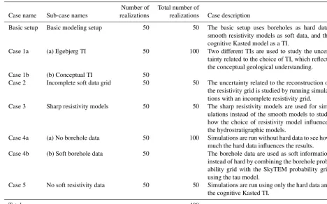
Figure 1.The Kasted survey area and resistivity–hydrostratigraphic relationship histograms.(a)shows the geographical location of the Kasted survey area and the Egebjerg model used as a secondary TI.(b)shows the reconstructed resistivity–hydrostratigraphic rela-tionship histograms for the three main hydrostratigraphic unit cate-gories based on SkyTEM resistivity models and borehole lithology logs.(c)shows the Kasted survey with the SkyTEM sounding and borehole locations. Note that the SkyTEM soundings are sampled so densely that the dots marking each individual sounding merge into blue lines.
the uncertainty related to stochastic hydrostratigraphic mod-eling using MPS methods.
3 Methods
3.1 Multiple-point statistics (MPS)
The multiple-point statistics framework stems from the gen-eral geostatistics framework. Here, multiple-point (MP) in-formation from a training image is used to condition simu-lations to probable geological patterns (Journel and Zhang, 2007). The TI thus provides a conceptual geological under-standing of a given area and can be viewed as a database containing probable geological patterns, which are used to condition the MPS simulation. The choice of TI is an im-portant step in any MPS setup and influences the realization results, as will be illustrated. The TI does not need to carry locally accurate information – i.e., the TI does not need to spatially or geographically overlap with real-world geologi-cal units – and can be purely conceptual in nature. Together with the TI, it is also possible to use geophysical datasets for constraining MPS simulations, resulting in realizations that reflect real-world regional geology. Today, MPS is a widely used tool, which is used in a variety of geoscience fields, including, but not limited to, reservoir modeling (e.g., Ok-abe and Blunt, 2004; Strebelle and Journel, 2001), hydrology (e.g., Le Coz et al., 2011; Hermans et al., 2015; Høyer et al., 2017), and geological modeling (e.g., de Iaco and Maggio, 2011).
3.1.1 Single normal equation simulation (snesim) The MPS method used in this paper is known as the sin-gle normal equation simulation (snesim) framework (Stre-belle, 2002), and is implemented in the Stanford Geosta-tistical Modeling Software, or SGeMS. The snesim frame-work allows for simulating a real-world categorical geolog-ical model using a TI, constrained using soft geophysgeolog-ical data and hard borehole data. The snesim algorithm scans the entire TI, ahead of simulation, and stores the MP informa-tion contained in the TI in a search-tree database. The MP information can then be retrieved from the database dur-ing simulation. The integration of soft geophysical data for constraining the simulations is achieved by utilizing the tau model, which will be described in detail in Sect. 3.2 (Journel, 2002; Krishnan, 2004). Here, the continuous soft data vari-able needs to be translated into a probability grid, describ-ing the probability of finddescrib-ing a given geological unit based on the geophysical data; see Barfod et al. (2018). In order to guarantee the reproduction of geological patterns at all scales, snesim uses the multiple-grid formulation, presented by Tran (1994).
3.1.2 Reconstructing incomplete datasets using direct sampling
In the field of geoscience, we are always dealing with in-complete datasets, since we cannot sample the subsurface exhaustively. Several approaches exist for dealing with
in-complete datasets, of which two general approaches can be defined. A common approach is to reconstruct incomplete datasets using geostatistical tools (e.g., Goovaerts, 1997; Ma-riethoz and Renard, 2010), which means that during the hy-drostratigraphic modeling process no information is present in the dataset gaps. However, it is important to emphasize that the reconstructed information is not as valuable as the actual measured geophysical information. The other common ap-proach is to just use the incomplete dataset as is. This means that no information is present in the dataset gaps during the hydrostratigraphic modeling process, which, depending on the modeling method, might result in large uncertainties.
In this study the MPS method called direct sampling (DS) is used for stochastic reconstruction of incomplete datasets (Mariethoz and Renard, 2010). The DS method uses the dataset we wish to reconstruct both as a simulation grid and a TI. This means that the patterns that are present in the incomplete dataset are inserted into the simulation grid be-fore reconstruction. It is, according to Mariethoz and Re-nard (2010), important that the patterns we wish to recon-struct are actually present in the incomplete dataset, since we are borrowing the patterns from the TI, or incomplete dataset, to stochastically reconstruct the dataset. If the patterns are not present in the incomplete dataset they will, simply put, not be inferred in the reconstructed dataset. Provided that enough information on the overall patterns is available in the incom-plete dataset, the DS method is a straightforward approach for reconstructing incomplete datasets.
3.2 The tau model: combining conditional probabilities Combining information from different sources is a frequent challenge in subsurface modeling. A fundamental challenge of the research conducted in this paper was to combine con-ditional probabilities from different sources. In this paper we used the common tau model approach (Journel, 2002). The tau model generally combines the probability values from different sources using Bayes’ theorem and a set of τ val-ues, orτ weights, for determining how to weigh the proba-bilities. The choice ofτ weights is subjective, and assigning these is not a trivial task. It is recommended to run a series of exhaustive tests when assigning theτ weights.
We will now briefly introduce the tau model; for more de-tails see Journel (2002). Firstly, we define a data event,Di, as a location vector,u, and a data value. Suppose we have a set of such data events,Dii=1, . . . ,n, and the goal is to estimate the probability that a hydrostratigraphic unit (A) is present provided all data events:
P (A|D1, . . .,Dn) . (1)
will consider D1 and D2 as 2-D or 3-D probability grids from different sources. As an exampleD1could be a prob-ability grid from geophysical data andD2a probability grid from borehole lithology logs. The probability grids are trans-lated into distance grids by applying the “probability-into-distance” transform:
xo=1−P (A) P (A) , x1=
1−P (A|D1) P (A|D1)
,
andx2=
1−P (A|D2) P (A|D2)
. (2)
Then the following distance ratio is computed using the tau model expression:
x x0 = n=2 Y i=1 xi x0 τi
, τ [−∞; +∞], (3)
where the tau values are [τ1,τ2]. The final conditional prob-ability is computed as follows:
P (A|D1,D2)= 1
1+x, (4)
where the value ofxis computed from Eq. (2), as follows: x=x0·
x 1 x0 τ1 · x 2 x0 τ2 . (5)
3.3 Comparing simulation results
[image:5.612.47.288.147.379.2]Comparing a large set of extensive 3-D models is a common problem encountered in stochastic MPS modeling. A com-mon approach is visual comparison, which is not an objective or quantitative comparison method. Each equiprobable hy-drostratigraphic model in this study contains 1 187 823 cells. Furthermore, a total of 400 MPS realizations were computed, Table 1, which makes it difficult to visually compare model-ing results. This, along with advances in stochastic modelmodel-ing tools such as MPS, motivated Tan et al. (2014) to develop a framework in which multiple 2-D or 3-D realizations can be compared quantitatively. The idea is to use a distance mea-sure, which measures the distance between two realizations. Realizations which are geometrically similar have small tance values, while dissimilar realizations have a large dis-tance value. The comparison techniques in this study are based on the principles presented by Tan et al. (2014). In this study the distances between individual realizations are based on the Euclidean distance transforms (Maurer et al., 2003). The usage of EDT as a measure for similarity will be described in more detail below. A full distance matrix is com-puted containing distances between each individual realiza-tion for all the different cases. The resulting 400 by 400 dis-tance matrix is then interpreted by itself.
3.3.1 Ensemble mode ratio maps (EMR maps)
The visual comparison can be helped by creating so-called ensemble mode ratio maps, or EMR maps. The idea is to
create a summary map portraying the mode ratio of a given ensemble of models, ranging between 1/Kand 1, whereKis the number of hydrostratigraphic categories. The EMR maps describe the certainty of the simulation based on the result-ing realization ensemble. If the EMR map shows a value of 1, then every single realization in the present ensemble has sim-ulated the same category or, in this case, hydrostratigraphic unit. On the other hand, if the EMR map shows a ratio of 1/K the ensemble of realizations shows equal probability for each of theKcategories. Each realization is equiprobable, and the EMR values of the categorical variables are computed from the probability distribution of a given cell with location,u. The probability that the attributeS is equal tosk,Pk(u), is computed as follows:
Pk(u)= 1 N
XN
i=1 sk,i(u)=sk
, (6)
whereN is the number of realizations,sk is the state of at-tributeSfor which we are currently computing the probabil-ity, andsk,i(u)is the state of the attribute at locationuand for theith realization. The EMR values for a given cell,u, can then be computed as follows:
rEMR(u)=(Pk(u)) , (7)
wherePk(u)denotes the probability for categoryk at loca-tionucomputed using Eq. (6).
The EMR values are then computed for each grid cell us-ing Eqs. (6) and (7), which, simply put, is the occurrence ratio of the mode category of a given ensemble containing a given number of realizations,Nreals. In other words, at a given location,u, if 45 out of 50 realizations yield the same category, then the EMR value is 0.9, and the ensemble cer-tainty for the given cell is high. On the other hand, with three possible lithological categories, i.e.,K=3, the lowest pos-sible certainty is 1/K=1/3, which means there is an equal probability of occurrence for each lithological category. This means that P (s1)=P (s2)=P (s3)=1/3, and therefore at the given location,u, therEMR=1/3 and the simulation is uncertain.
3.3.2 Euclidean distance transforms (EDT) – measuring similarity between 3-D hydrostratigraphic realizations
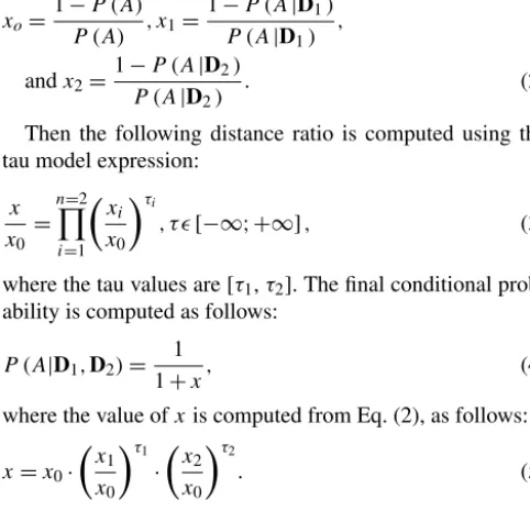
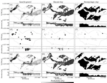
Figure 2.A 2-D example of the Euclidean distance transforms (EDT) as a measure for the similarity between categorical MPS realizations. In this example a set of 50 realizations, from the basic modeling setup, are compared based on the differences in EDT for sand and gravel units.(a–d)show the hydrostratigraphic models for the TI, closest realization, 25th closest realizations, and farthest realization, respectively.
(e–h)show, in the same order as above, the binary images of the sand and gravel units of the 2-D hydrostratigraphic model layers.(i–l)show, in the same order as above, the Euclidean distances layers computed from the 2-D sand and gravel binary layers.
the medium depicted by the state code 1, i.e., for grid cell at locationu:
dEDT(u)=(ku−vk2) , (8)
wherevis a set of grid cells with a state code equal to 1. The dEDT implementation presented by Maurer et al. (2003) uses a computationally favorable method for com-puting the exhaustive EDT at all locations in a binary grid.
To illustrate thedEDTapproach for comparing realizations a 2-D example case is presented. The basic modeling setup contains 50 realizations, i.e.,Nrealizations=50, which are go-ing to be compared to the cognitive model, which in this case also happens to be the TI. The 2-D example is cre-ated by selecting the horizontal cross section at 20 m b.s.l., for each of the 50 basic modeling setup realizations and the single cognitive geological model (Fig. 2a–d). Each of the 2-D layers are transformed into 2-2-D binary layers, portraying sand and gravel as the main variable, and glacial clay and hemipelagic clay as a background variable (Fig. 2e–h). The 2-D binary layers are then translated into 2-DdEDTlayers by using Eq. (8) to exhaustively compute thedEDTat each grid cell for all of the 50 realizations. The resultingdEDTlayers, of which three are seen in Fig. 2i–l, are used to compute an average Euclidean distance between each realization, mr,i, and the cognitive geological model,mcog:
1dEDT mcog, mr,i
= 1
M XM
j=1
h dEDTmcog uj
−dmr,i
EDT uj
i , (9)
wherei∈ {1, . . ., N}, withN being the number of realiza-tions, which in this case isN=50, andMbeing the number of cells in the simulation grid, or in this case, the 2-D layer. The 1dEDT, Eq. (9), then describes the average difference of the distance to the nearest active cell in the binary grid. The 50 realizations are then ranked by the average Euclidean distance differences,1dEDT, as seen in Fig. 2, where the re-alization which is closest to the cognitive geological model (Fig. 2b, f and j) has a1dEDTvalue of 240 m, the realization which was ranked 25th closest (Fig. 2c, g and k) has a1dEDT value of 280 m, and lastly the realization which was farthest (Fig. 2d, h and l) has a1dEDTvalue of 310 m. It should be noted that the1dEDT computation, described by Eq. (9), is not limited to comparing a realization to a cognitive model and can in fact be used to compare any pair of 3-D categor-ical models. In fact, a generalized version of Eq. (9) can be defined as follows:
1dEDT(mA, mB)=
1 M
XM
j=1
dmA
EDT uj
−dmB
EDT uj
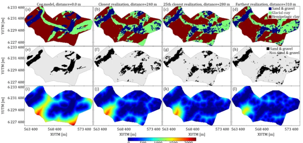
Figure 3. A schematic diagram presenting the conversion of the lithological logs into probability logs for the three hydrostrati-graphic units: sand and gravel, glacial clay, and hemipelagic clay. Step 1: the lithology log is translated into a hydrostratigraphic log. Step 2: the hydrostratigraphic logs are resampled according to the vertical modeling grid intervals and an interval probability is calcu-lated for each of the hydrostratigraphic units.
distance for each of the three hydrostratigraphic categories, ensuring that the distance values reflect the complexities re-lated to each of the hydrostratigraphic categories.
3.3.3 Evaluating the distance matrix
The average Euclidean distance difference, 1dEDT, from here on referred to as the distance between two realizations, is exhaustively computed between all realizations and com-piled into an exhaustive 400 by 400 distance matrix. The dis-tance matrix,D, contains all distance values between all hy-drostratigraphic realizations computed using Eq. (9) and is defined as follows:
Di,j =dEDT mr,i, mr,j, (11)
whereij= {1, . . ., N}, withN being the number of realiza-tions. The distance matrix, D, can be evaluated directly by comparing the distances between individual realizations to
each other. Another option is to summarize the distance ma-trix in a table representing the distances between the differ-ent cases. This is achieved by organizing the distance matrix according to which case they belong to. In this study the dis-tance matrix is sorted according to the order of the individual cases, as in Table 1. The distance matrix can then be sum-marized by computing the average distance for each group of realizations pertaining to a specific case. The concepts of distance variability and distance to cognitive model were pre-sented by Barfod et al. (2018) and are also used here. The concept is that the variability pertaining to a specific case can be determined by computing the average of the distances of the 50 realizations for a given case ensemble. Another mea-sure is the distance to the cognitive model. The distances be-tween all realizations and the cognitive model are computed, and this provides a reference point to which the realizations are compared.
4 MPS modeling setup
and Table 1 summarizes each case. First of all, the model discretization and parameterization as well as construction of hard and soft data grids are described.
The Kasted model covers an area of 12 km by 7 km, dis-cretized on a modeling grid with 229 by 133 by 39 cells, containing a total of 1 187 823 cells. Each cell has a size of 50 m by 50 m by 5 m. It is parameterized into three hydros-tratigraphic units, listed as follows.
1. Sand and gravel: a combination of coarse lithological units, including sand till, meltwater sand, gravel and pebbles of glacial origin, late glacial freshwater sand, and postglacial freshwater sand.
2. Glacial clay: this category contains silty and sandy clays, including clay till and meltwater clay of glacial origin.
3. Hemipelagic clay: a combination of fine grained con-ductive clays, containing the extensive and homo-geneous hemipelagic Paleogene and Oligocene clays found in Denmark.
These three categories serve the purpose of simplifying the geology of the Kasted area. The Kasted survey lithology logs reveal a combination of 59 geological categories, which are translated into a set of hydrostratigraphic logs (Step 1, Fig. 3) using these hydrostratigraphic categories. Similarly, the 42 geological units in the cognitive geological model are di-vided into the three abovementioned categories (Fig. 4a). The vertical proportions of the three-category hydrostratigraphic Kasted model can be viewed in Fig. 5a.
The borehole lithology logs need to be assigned to a 3-D grid, which is carried out in three overall steps. The first step is to translate the borehole lithology logs into hydros-tratigraphic logs using the above mentioned three categories; Step 1, Fig. 3. The second step is then to divide the hydros-tratigraphic logs into intervals identical to the vertical inter-vals of the model grid. At each resampled interval a proba-bility value is directly calculated for each hydrostratigraphic unit; Step 2, Fig. 3. The probability is simply the percent-age of the given unit, which is present within the interval. Finally, the last step is to assign the hydrostratigraphic prob-abilities to a grid. The probability values are assigned to the grid cell in which the given hydrostratigraphic log is present. On the rare occasion that multiple logs are present within a given cell, the probabilities are combined accordingly to one representative probability value. The end result is a grid con-taining the borehole probability values of each hydrostrati-graphic unit: sand and gravel, glacial clay, and hemipelagic clay. It is common to view borehole lithology logs as hard information, or ground truth. The borehole probability grid can therefore be translated into a hard data grid, by assigning the most probable hydrostratigraphic unit in each grid cell.
[image:8.612.326.524.68.567.2]The 1-D SkyTEM resistivity models are assigned to a 3-D grid, identical to the modeling grid. The first step is to fill all
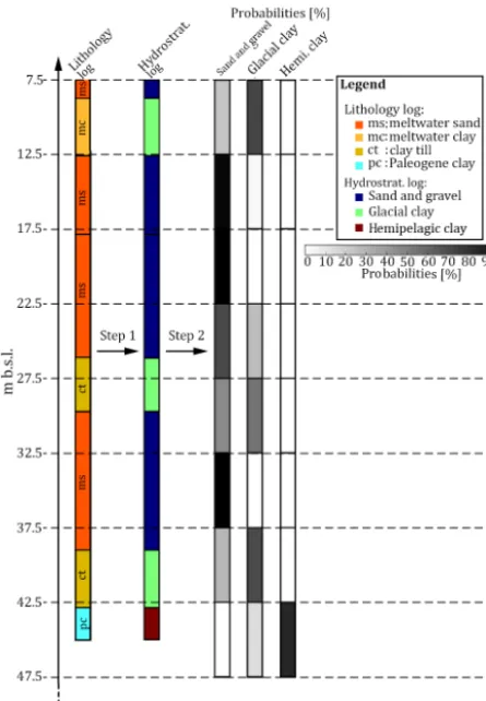
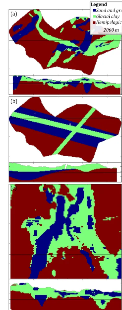
Figure 4.An overview of the training images (TIs) which are used during MPS simulation. A horizontal slice and vertical cross sec-tion is presented for each TI, portraying the hydrostratigraphic ar-chitecture;(a)shows the Kasted TI,(b)shows the conceptual TI, and(c)shows the Egebjerg TI, which is generally larger than the Kasted model.
re-sistivity grid using DS stochastic reconstruction (Mariethoz and Renard, 2010) (Fig. 7). The reconstruction procedure was originally presented by Barfod et al. (2018); however, we have made some improvements for this study. Originally, a simple kriging estimation approach was used to assign the resistivity models to a 3-D modeling grid. This resulted in an incomplete resistivity grid, which contained resistivity infor-mation not only pertaining to grid cells containing a SkyTEM sounding; i.e., the resistivity grid had already been partly re-constructed in the proximity of the geophysical soundings. To avoid this, block kriging estimation was used instead. The block kriging method is also a variogram-based estimation method, which estimates the average value of a rectangular block (Goovaerts, 1997). For more details on reconstructing incomplete resistivity grids see Barfod et al. (2018).
The SGeMS snesim framework utilizes the tau model for soft data conditioning (Journel, 2002), which re-quires the translation of resistivity grids into probability grids. This requires information on the regional resistivity– hydrostratigraphic relationship. Such knowledge is not al-ways available, but if enough boreholes and electromag-netic geophysical data are available, the framework for study-ing the resistivity–hydrostratigraphic relationship, presented by Barfod et al. (2016), can be used to create a set of histograms. The resistivity–hydrostratigraphic histograms, Fig. 1b, are compiled from available hydrostratigraphic logs and SkyTEM resistivity models and are presented in more detail in Barfod et al. (2016, 2018). The estimated histograms (Fig. 1b) are then used to directly translate each resistivity value, in a given resistivity grid, into three probabilities, one for each hydrostratigraphic unit.
The general MPS workflow can be summarized in seven overall steps as follows:
1. Using block kriging, the SkyTEM resistivity models are assigned to a 3-D grid identical to the Kasted model grid.
2. The incomplete resistivity grids (Fig. 6a) are stochasti-cally reconstructed using direct sampling (Fig. 7a). The result is an ensemble of 50 equiprobable reconstructed resistivity grids.
3. The reconstructed resistivity grids are trans-lated into probability grids using the resistivity– hydrostratigraphic relationship histograms (Fig. 1b). 4. The borehole lithology logs are translated into
hydros-tratigraphic logs; Step 1, Fig. 3.
5. The hydrostratigraphic logs are resampled and three probability values, one for each hydrostratigraphic unit, are directly computed at each resampled interval; Step 2, Fig. 3.
6. The borehole probabilities are assigned to a grid identi-cal to the cognitive Kasted model grid.
7. The borehole probability grid is translated into a hard data grid, by assigning the most likely hydrostrati-graphic unit to each grid cell.
A total of 400 realizations are created, with 50 realiza-tions per sub-case (Table 1). In snesim a random number seed needs to be manually selected for each realization to initialize the random number generator and in particular define a ran-dom path through the modeling grid. The ranran-dom seed con-vention chosen in this paper was to apply the same random seed vector to each sub-case. The vector contains 50 linearly increasing random seed numbers, ensuring consistency when comparing realizations from the individual sub-cases. 4.1 Basic modeling setup
The basic modeling setup is designed to act as the base from which all other cases are built. The different sub-cases are simply modified versions of the basic modeling setup, each designed to study how modification to the base setup relates to hydrostratigraphic MPS modeling. The basic modeling setup uses the borehole data as hard information, SCI models with smooth inversion constraints as soft data, and the cog-nitive hydrostratigraphic Kasted model as a TI (Fig. 4a), for which the global proportions are listed in Table 2 and vertical proportions are displayed in Fig. 5a.
4.2 Case 1 – conceptual geological understanding The basic modeling setup uses the actual cognitive geolog-ical model of the Kasted survey area as a TI (Høyer et al., 2015). In Denmark, it is common practice to build 3-D cog-nitive geological models of the near-subsurface. Many cogni-tive models exist and are publicly available. Such models can easily be adapted and used as 3-D TIs to simulate new survey areas, provided the geological settings are similar. Case 1 is divided into two sub-cases. The first sub-case, case 1a, uses the basic setup, but, in place of the cognitive Kasted model, the cognitive geological model of the Egebjerg area (Fig. 1a) is used as a TI (Fig. 4c). The geologic setting in Egebjerg is relevant since it is partly dominated by a buried valley com-plex (Jørgensen et al., 2010).
Table 1.An overview table showing information on the MPS cases along with information on the number of realizations for each case or sub-case, and a brief description of each case.
Number of Total number of
Case name Sub-case names realizations realizations Case description
Basic setup Basic modeling setup 50 50 The basic setup uses boreholes as hard data, smooth resistivity models as soft data, and the cognitive Kasted model as a TI.
Case 1a (a) Egebjerg TI 50 100 Two different TIs are used to study the uncer-tainty related to the choice of TI, which reflects the conceptual geological understanding. Case 1b (b) Conceptual TI 50
Case 2 Incomplete soft data grid 50 50 The uncertainty related to the reconstruction of the resistivity grid is studied by running simula-tions with an incomplete resistivity grid. Case 3 Sharp resistivity models 50 50 The sharp resistivity models are used for
sim-ulations instead of the smooth models to study how the choice of resistivity model influences the hydrostratigraphic models.
Case 4a (a) No borehole data 50 100 Simulations are run without hard data to see how much the hard data influences the results. Case 4b (b) Soft borehole data 50 The borehole data are used as soft information
instead of hard by combining the borehole prob-ability grid with the SkyTEM probprob-ability grid using the tau model.
Case 5 No soft resistivity data 50 50 Simulations are run using only the hard data and the cognitive Kasted TI.
Total – – 400 –
Table 2. The global proportions related to each of the three TIs presented in Fig. 4.
Sand and Glacial Hemipelagic gravel clay clay Kasted TI 0.17 0.21 0.62 Conceptual TI 0.17 0.22 0.61 Egebjerg TI 0.10 0.22 0.68
contains coarse, block-like geological features. The impor-tant features, in relation to hydrostratigraphic modeling, are the buried valley complexes, which are present in the Egeb-jerg model (Fig. 4c). The global proportions of the EgebEgeb-jerg TI (Table 2) are similar to the ones found in the Kasted TI. However, the vertical proportions of the Egebjerg TI (Fig. 5c) are different, especially in the upper part of the TI where glacial clay units dominate.
The second sub-case, case 1b, utilizes a purely conceptual TI. The conceptual TI is created by using a set of hyperbolic secant functions to populate a 3-D matrix and is purely math-ematical in nature. The conceptual TI can be seen in Fig. 4b and is designed to have three overall buried valleys eroded into a hemipelagic clay substratum. There are two narrow and shallow glacial clay valleys, and a broad and deep sand
and gravel valley. One of the glacial clay valleys is a younger valley that is eroded into the older sand and gravel valley and they run roughly parallel to each other. The last glacial clay valley is almost orthogonal to the other valleys, and also erodes into the sand and gravel valley. The upper part of the TI contains a cover layer of glacial clay (Fig. 5b). The sim-ple conceptual TI is designed to contain the main geologi-cal architecture of the Kasted area, namely the buried val-ley complexes. The sand and gravel valval-ley, trending west– northwest to east–southeast, was chosen on purpose to study what happens when oversimplified and smooth MP informa-tion is added to a TI. The global proporinforma-tions of the concep-tual TI are consistent with the other TIs, while the vertical proportions for sand and gravel and glacial clay units show a significantly different pattern (Fig. 5b).
4.3 Case 2 – incomplete soft data
[image:10.612.65.269.445.511.2]Figure 5.The vertical proportions of the three training images for each of the hydrostratigraphic categories, where (a)portrays the Kasted TI,(b)the conceptual TI, and(c)the Egebjerg TI.
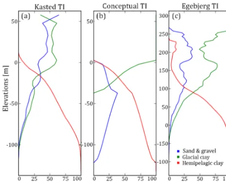
reconstruct missing patterns is present. Signs of mediocre data density are seen in the incomplete grids (Fig. 6a). Ar-tifacts from the DS reconstruction are present in the com-pleted resistivity grids. The resistive valley to the west in the horizontal slices and vertical cross sections in Fig. 7a and b reveal a striated pattern. An alternative to reconstructing the resistivity grid beforehand is to use the incomplete resistiv-ity grids for simulation, meaning no information is present in the resistivity dataset gaps. Grid cells containing a resis-tivity model are translated into three probability values us-ing the resistivity–hydrostratigraphic relationship histograms (Fig. 1b, 6b–d). Areas without soft resistivity data rely on the TI during simulation, emphasizing the fact that no actual in-formation is present between soundings. The overall setup is identical to the basic setup; the only difference is the recon-structed soft data grids are interchanged for the incomplete soft data grid (Fig. 6b–d).
4.4 Case 3 – choice of resistivity model
The choice of inversion algorithm results in different SkyTEM resistivity models. The purpose of this case is to study how using sSCI (Vignoli et al., 2015) models influ-ences the modeling results. A common inversion approach is SCI, where a smooth regularization is used (Constable et al., 1987). Such resistivity models have a smooth transition from resistive to conductive features, and vice versa. Geological layer boundaries are rarely smooth in nature, meaning such soft transitions in resistivities seldom reflect reality. Further-more, extreme resistivity values are not presented correctly in the smooth model inversions. Vignoli et al. (2015) propose an alternative SCI approach, employing a minimum gradi-ent support regularization term instead. Such sSCI models
produce resistivity models with sharp layer boundaries and a better representation of extreme values. The setup in case 3 is identical to the basic setup, except that the SCI models are interchanged for sSCI models. The DS grid reconstruction is then conducted on the sSCI models, which are then trans-lated into probability grids. Finally, these grids are used as soft data for simulation using the snesim method.
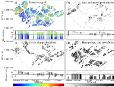
The sharp resistivity models are different from the smooth models, but no particularly sharp layer boundaries are re-flected in the reconstructed resistivity grid (Fig. 7b).
One of the obvious differences is found in the resistivity patterns of the sand and gravel valley to the far west of the survey area. The valley itself is not significantly different; however, the small resistive patch, west of the large valley, is more pronounced in the sharp model and has an overall more pronounced fingerprint (Fig. 7b). The sharp resistivity mod-els better estimate the true bulk resistivity values of specific geological units, such as the resistive patch accentuated here. The ensemble standard deviation grid, Fig. 7c and d, shows a general reduction in the ambiguity of the reconstructed sharp resistivity models. This is clear from the reduction areas with large standard deviation, shown in red colors, which are over-all reduced in size.
4.5 Case 4 – borehole lithology logs
This case is dedicated towards how the borehole data are handled and how they influence the hydrostratigraphic mod-eling results. The hard borehole data are normally sparse, relative to geophysical data. Boreholes are commonly con-sidered ground truth since they directly sample the subsur-face sediments or petrological units. This case is divided into two sub-cases. The first sub-case, case 4a, portrays what hap-pens when hard data are not included in the snesim simula-tion. The model setup is therefore identical to the basic MPS setup, but without including the borehole data.
Figure 6.A presentation of the incomplete resistivity grid. Each grid is portrayed as a horizontal slice at 20 m b.s.l. and a vertical cross section intersecting at YUTM 6 230 100 m.(a)shows the resistivity grid which is translated into three probability grids using the resistivity– hydrostratigraphic relationship histograms (Fig. 1b). Grid cells without SkyTEM soundings are not assigned a probability value.(b–d)show the sand and gravel, glacial clay, and hemipelagic clay probability values, respectively.
in this case is the vertical proportion taken from each layer of the cognitive Kasted TI (Fig. 5a). Then the probability dis-tributions are defined as follows: P (A|Dr) andP (A|Db), whereDris the resistivity probability grid andDbthe bore-hole probability grid. The 3-D probability grids are translated into distance grids by applying the probability-into-distance transform and computing the distance ratio using Eqs. (2) and (3), where the tau values were assigned based on a se-ries of exhaustive tests. The final tau values were selected based on the criteria that the transitions in areas where both borehole and resistivity information is available should be as smooth as possible in the resulting combined probability grid, as seen in Fig. 8. Based on the tests, the resulting tau values were [τr, τb]=[2.0,1.0]. The final conditional prob-ability was computed using Eq. (4) and resulted in the three hydrostratigraphic probability grids, as seen in Fig. 8g–i. The combined probability grids replace the smooth probability grids used in the basic setup.
4.6 Case 5 – excluding the soft resistivity data
The final case, case 5, illustrates the consequences of not in-cluding the soft SkyTEM resistivity information in the MPS simulation routine. The basic setup is simply run without the
inclusion of soft data; i.e., the setup only uses the cognitive Kasted TI and hard borehole information.
5 Results
5.1 Visual comparison of hydrostratigraphic realizations and ensemble mode ratio maps
hy-Figure 7.An overview of the key differences between reconstructing the resistivity grid using smooth and sharp inversion resistivity models. Each grid is portrayed as a horizontal slice at 20 m b.s.l. and a vertical cross section intersecting at YUTM 6 230 100 m.(a)shows the smooth reconstructed resistivity grid.(b)portrays the sharp reconstructed resistivity grid.(c)shows the standard deviation calculated from 50 stochastic reconstructions of the smooth resistivity grid.(d)shows the standard deviation calculated from 50 stochastic reconstructions of the sharp resistivity grid.
drostratigraphic units. The basic modeling setup realizations reveal sporadic and random patterns. The sand and gravel units are placed in small lumps throughout the glacial clay units, but are not present within the homogenous hemipelagic clay. Patches of uncertain glacial clay units are, however, found in the homogeneous hemipelagic clay, especially in the southeast corner of the Kasted survey area (Figs. 9a, 10a). The same sporadic picture is seen in the vertical slices of the realizations (Fig. 9a), although here an additional trend is revealed. The sand and gravel valley to the far west and at XUTM 570 900 m is not consistently filled with sand and gravel (Fig. 9a) as in the cognitive geological model (Fig. 4a). Furthermore, the EMR map reveals that the valley margins are subject to a larger degree of ambiguity (Fig. 10a); in fact at some locations therEMRvalue is close to 1/3, which means that for the model ensemble the occurrence of either hydrostratigraphic unit is possible.
The case 1a realizations (Fig. 9b, 10b), which use the Egebjerg TI (Fig. 4c), show the same overall trends as in the basic modeling setup. The subset of buried valleys men-tioned above is present; however, an obvious difference is the coarse and block-like appearance of the case 1a realization ensemble. This appearance is similar to the block-like ap-pearance of the Egebjerg TI (Fig. 4c). Furthermore, the hori-zontal slice of the realizations and EMR map reveals that the glacial-clay-dominated area to the east has a generally larger
occurrence ratio and is thus more certain. The realizations are clearly influenced by the choice of TI, especially when case 1b is also considered (Fig. 9c). The hydrostratigraphic realizations of case 1b (Fig. 9c, 10c) clearly depict the same overall buried valley trends, but the valleys in the central part of the model are largely filled with the opposite of the valley filling hydrostratigraphic units. Furthermore, the occurrence ratio seems quite low in certain areas, such as to the south of the model, which means the ambiguity has increased. Fi-nally, the realizations also reveal an absence of small-scale patterns, which corresponds to the conceptual TI that only contains homogenous hydrostratigraphic units.
The importance of reconstructing the incomplete resistiv-ity grid is seen in case 2 (Fig. 9d, 10d). The two realiza-tions in Fig. 9d show the main buried valley features, e.g., the western sand and gravel valley. However, the hydrostrati-graphic units are sporadic, especially in areas with no data. Patches of sand and gravel and glacial clay are randomly spread throughout the presented horizontal slice and verti-cal cross section (Fig. 9d). The EMR map also reveals an increase in low occurrence ratios in areas without soft data (Fig. 10d).
[image:13.612.120.479.69.313.2]mod-Figure 8.A visual representation of the tau model procedure for combining the soft resistivity and borehole grids. Each grid is portrayed as a horizontal slice at 20 m b.s.l. and a vertical cross section intersecting at YUTM 6 230 100 m.(a–c)show the sand and gravel, glacial clay, and hemipelagic clay probability maps, respectively, for one DS reconstructed resistivity grid;d–fshow the 200 m radius kriged borehole probability; and(g–i)show the combined resistivity grid, which has been combined using a tau model with the values[τr, τb] =[2, 1].
eling setup realizations (Fig. 9a). However, a key difference is the significant reduction or absence of patches of glacial clay in the homogeneous hemipelagic clay. In fact only one patch is found in the first realization (Fig. 9e) in the south-west corner, while it is not present in the second realization, and the EMR map further reveals a reduction of the occur-rence ratios generally, especially along the southern margin of the realizations (Fig. 10e).
Case 4 shows the influence that the hard data have on the hydrostratigraphic realizations in two sub-cases: case 4a, where snesim simulations are run without hard data; and case 4b, where the borehole data are treated as soft infor-mation. Fig. 9f and g shows two hydrostratigraphic realiza-tions without hard data and with soft borehole data, respec-tively. These realizations do not differ significantly from the basic modeling setup realizations and in fact are quite simi-lar. One key difference is the central glacial clay valley strik-ing ∼E30◦S, which does not contain any sand and gravel to the west (Fig. 9f and g). The EMR maps reveal that with-out boreholes (Fig. 10f) the occurrence ratios generally de-crease, making the realizations more ambiguous. The usage of the borehole data as soft information also seems to reduce the occurrence ratios compared to the basic modeling setup. Generally, leaving out the borehole data, or treating it as soft
data, results in local changes in areas with a high density of boreholes.
The final case, case 5, illustrates the importance of the SkyTEM soft data. The snesim simulations are run using only hard data and the cognitive geological model as a TI. The output realizations (Fig. 9h) portray smooth and large-scale hydrostratigraphic units. The hydrostratigraphic archi-tecture of the buried valleys is not reflected. However, the sand and gravel valley, to the west, does seem to protrude slightly in the realizations (Fig. 9h) and the EMR map reveals a significant decrease in the occurrence ratio and thus an in-crease in the ambiguity of the model ensemble (Fig. 10h). 5.2 Quantitative comparison using differences in
object-based Euclidean distances as a measure for similarity
[image:14.612.118.484.67.353.2]Figure 9.Each case is displayed by two realizations: realization no. 1 of 50 and realization no. 30 of 50. Each realization is portrayed as a horizontal slice at 20 m b.s.l. and a vertical cross section intersecting at YUTM 6230100 m.(a)shows the realization results for the basic modeling setup,(b)shows the realization results for case 1a,(c)shows the realization results for case 1b,(d)shows the results for case 2,
(e)shows the results for case 3,(f)shows the results for case 4a,(g)shows the results for case 4b, and(h)shows the results for case 5. For more details on individual cases the reader is referred to Table 1.
The basic modeling setup constitutes a common snesim setup, with the geophysical data as soft data, boreholes as hard data, and a 3-D geological conceptualization encased in a TI. The ensemble average variability is computed accord-ing to the equations presented by Barfod et al. (2018), and the resulting ensemble average variability is 10.1 m, with an av-erage distance to the cognitive model of 24.3 m. This means that the Euclidean distance mismatch between the individual realizations related to basic modeling setup is 10.1 m, and the average difference in Euclidean distance to the nearest active cell between the realizations and the cognitive model was 24.3 m.
The 3-D geological conceptualization contained in the TI influences the final hydrostratigraphic realizations as illus-trated in case 1, which is divided into two sub-cases: case 1a and case 1b. In case 1a, using a 3-D cognitive geological model from the Egebjerg area as a TI for hydrostratigraphic simulation increases the average distance to the cognitive model to 24.9 m (Fig. 11a, Table 3). Furthermore, the average
variability has increased to 13.6 m (Fig. 11b, Table 3). The other sub-case revolves around using an entirely conceptual geological model as a TI. The conceptual TI was designed to reflect the overall geology, yet still contains some bias. The results reflect the bias, with increased distances to the cog-nitive geological model, which are now centered on 25.6 m (Fig. 11a, Table 3). The ensemble variability has increased to 14.8 m (Fig. 11b, Table 3).
The importance of proper reconstruction of the incomplete resistivity grid is illustrated in case 2, where the incomplete resistivity grid was used for simulation. The resulting real-ization ensemble has a large ensemble variability centered on 24.1 m (Fig. 11a, Table 3). The distance to the cognitive ge-ological model is also large, with an average value of 33.1 m (Fig. 11b, Table 3).
Figure 10.A presentation of the ensemble mode ratio (EMR) maps, computed for the different case ensembles of hydrostratigraphic models. Each EMR map is presented as a horizontal slice centered on 20 m b.s.l. and a vertical cross section intersecting at YUTM 6 230 150 m.(a–h)present the EMR-type uncertainty map for each of the different cases, which are summarized in Table 1. The EMR values portray how certain the ensemble of MPS realizations are; i.e., ifrEMR=1/3 then the realization is uncertain, and we have
equal probability of finding either hydrostratigraphic unit since
P (s1)=P (s2)=P (s3)=33 %. On the other hand, if rEMR=1,
then each realization of the given ensemble contains the same hy-drostratigraphic unit at the given grid cell.
realization ensemble, i.e., the distances between the realiza-tions pertaining to case 3, is small, with an average value of 9.4 m – see Table 3. Recalling the raw hydrostratigraphic re-alizations (Fig. 9e) and the EMR map (Fig. 10e), the large reduction in distances could partly be related to the removal of non-hemipelagic clay units along the southern border of the model and an overall increase in confidence along the southern and southeastern border of the model.
The influence of the borehole lithology logs on the hy-drostratigraphic realizations is reflected in case 4, which is divided into two sub-cases. In the first sub-case, case 4a, the
borehole information is not used as hard data, and the real-izations are created only using soft geophysical data and the Kasted TI. However, the borehole data are still used for cre-ating the resistivity–hydrostratigraphic histograms (Fig. 1b), which are used for creating the probability grids. The ensem-ble average variability is 10.7 m (Fig. 11a, Taensem-ble 3) and the average distance to the cognitive model is 24.3 m (Fig. 11b, Table 3). In the second sub-case, case 4b, the boreholes are used as soft information to reflect the uncertainty of the bore-hole information. The ensemble average variability is 10.9 m, and the average distance to the cognitive model is 24.3 m. This illustrates how the snesim realizations are not particu-larly sensitive towards the sparse borehole hard data.
Not including the geophysical soft data in the snesim sim-ulations, case 5, resulted in the largest ensemble average variability of 40.0 m (Fig. 11a, Table 3). The average dis-tance between case 5 realizations and the cognitive model was 59.3 m. This means that the realizations of case 5 are the most different from the rest of the realizations. The snesim realizations are sensitive towards not including the geophys-ical data, or using the incomplete resistivity grid. This under-lines the importance of the geophysical soft data in relation to hydrostratigraphic modeling using the snesim methodology.
6 Discussion
The cognitive geological model was created based on smooth SkyTEM resistivity models and lithological logs (Høyer et al., 2015) as well as the conceptual geological understand-ing of the area. The model was simplified from a full 3-D geological model containing a total of 42 unique geological units to a hydrostratigraphic model containing only 3 hydros-tratigraphic units. The cognitive geological model, although detailed and extensive, is not the true geological model. The ensemble realizations should not directly reflect the cogni-tive model, yet the cognicogni-tive model can be thought of as a reference point in modeling space, which we would prefer our models to resemble.
[image:16.612.52.286.65.416.2]Table 3.A summary table showing the average distance value for each 50 by 50 square representing a given case in the distance matrix (Fig. 11a). The final column, labeled Distancecog, summarizes the distances to the cognitive geological model, presented as the average
of each colored point cloud in Fig. 11b. The distances in parenthesis represent ensemble variabilities, and the remaining values represent average distances between different ensembles. The unit of the average distances is meter.
Distance (m) Basic setup Case 1a Case 1b Case 2 Case 3 Case 4a Case 4b Case 5 Distancecog
Basic setup (10.1) 12.9 16.9 24.0 12.7 11.1 11.2 49.6 24.3 Case 1a 12.9 (13.6) 18.3 26.0 15.1 14.0 13.9 51.7 24.9 Case 1b 16.9 18.3 (14.8) 27.9 17.8 18.1 18.1 52.5 25.6 Case 2 24.0 26.0 27.9 (24.1) 23.5 25.0 24.9 45.2 33.1 Case 3 12.7 15.1 17.8 23.5 (9.4) 13.6 13.6 49.6 21.6 Case 4a 11.1 14.0 18.1 25.0 13.6 (10.7) 11.1 50.7 24.3 Case 4b 11.2 13.9 18.1 24.9 13.6 11.1 (10.9) 50.6 24.3 Case 5 49.6 51.7 52.5 45.2 49.6 50.7 50.6 (40.0) 59.3
models to the modeling grid resulted in smoothing of sharp vertical boundaries otherwise found in sSCI models. These three cases together reveal the importance of the geophysical soft data when using the snesim setup presented in this study. In relation to case 5, it can be argued that, even though the SkyTEM resistivity models are not used as soft data, they are still included indirectly since the TI, or cognitive geological model, was created using smooth SkyTEM resistivity mod-els. However, the realizations related to case 5 revealed an ensemble of realizations, which did not replicate the overall geological architecture, implying the importance of using the SkyTEM models as soft data.
On the other hand, the cases related to studying the sen-sitivity towards borehole information, case 4a and case 4b, revealed that the large-scale hydrostratigraphic architecture was not changed significantly. The distance measure used in this study observes similarities or dissimilarities of large-scale hydrostratigraphic architecture and is not sensitive to-wards local changes in small-scale patterns. The amount of geophysical information is relatively large, meaning the rel-ative influence of (few) borehole data becomes less signifi-cant. This does not mean that the borehole data are not impor-tant; they both contain locally accurate information and are used to estimate the regional resistivity–hydrostratigraphic relationship (Fig. 1b). In other surveys, where the contrast between geophysical and lithological information is smaller, the importance of the borehole data will likely increase. In relation to this study, such small-scale changes are insignifi-cant. Yet if the realizations are to be used for flow simulations or predictions on a smaller scale, such smaller scales might suddenly have an important impact on prediction accuracy. Additionally, if such small-scale patterns are important, the size of the model grid cells should be smaller to accommo-date simulations of these variations. Discretizing hydrostrati-graphic and groundwater models with relatively small grid cells can be CPU demanding, depending on the total number of grid cells.
In case 4b, the borehole data were used as soft information as in the study by Høyer et al. (2017). This was done since
boreholes are associated with uncertainty related to a number of factors, as described above. Therefore, the soft borehole probability values derived during the assigning of the bore-holes to the modeling grid are combined with the SkyTEM-based probability grids using the tau model. This approach enables the borehole probability to alter the final probability grid, while still conditioning the SkyTEM data. Combining the information rather than letting the borehole data count as ground truth, i.e., hard data, allows the borehole data to influence the realizations, especially if the soft borehole in-formation disagrees with the soft geophysical data (Fig. 8).
Figure 11.A presentation of the average Euclidean distance calcu-lations.(a)shows the full distance matrix;(b)shows the average Euclidean distances between each individual hydrostratigraphic re-alization and the cognitive geological model.
model (Fig. 4a), is represented as sand and gravel. This leads to the conclusion that one needs to pay attention to the con-struction of the TI, as also witnessed in the study by Høyer et al. (2017). Furthermore, the large-scale and homogenous nature of the hydrostratigraphic architecture in the concep-tual TI results in realizations which reflects the homogeneity. In comparison with the realizations based on the TIs derived from cognitive models, the realizations contain much fewer small-scale patterns.
Small-scale patterns are present in the realizations al-though they are not at the same degree present in the TIs. This can be explained by the fact that the simulations are probabilistic in nature and are based on random processes. At the beginning of the simulation a random path is drawn so that the simulation grid is filled by visiting each grid cell
only once. The small-scale patterns are partly due to the hard data that are inserted into the simulation grid before the sim-ulation commences, which is excluded from the simsim-ulation path. As the grid is filled out, the hard borehole data might suggest a certain category but the soft data suggest another category. As the grid is filled out the overall category from the soft data dominates and, if the random path visits the grid cells near the hard data point towards the end of the random path, then we are left with a small intercalation (Hansen et al., 2018). The intercalations are also inherent in the sim-ulations without hard data, which is mainly due to process randomness related to how the snesim algorithm draws from a cumulative density function (Strebelle, 2002).
The Kasted model and TI are influenced by non-stationarity, which has not been dealt with in the MPS setup. Even though the models are influenced by non-stationarity, the simulations result in models which overall resemble the cognitive model, e.g., cases 1–4. However, once the geophys-ical data are removed in case 5, the resulting MPS mod-els are increasingly random and are heavily influenced by non-stationarity. It is important to note that the increasing amounts of soft geophysical data generally decrease the ef-fects of non-stationarity, due to the increased conditioning of the soft data.
The reconstruction of the resistivity grid is an important step of the MPS setup presented in this study. This was il-lustrated in case 2, where the incomplete resistivity grid was used instead of the reconstructed resistivity grid, resulting in larger realization variability and distance to the cognitive ge-ological model. These realizations could have been improved by increasing the prior knowledge provided to snesim before simulation. One such option is to provide so-called vertical proportions, in place of solely the target global proportions. The global proportions simply give a percentage fraction of the different hydrostratigraphic units in the outcome real-izations. The vertical proportions are defined for each sim-ulation grid layer and determine the proportions as a func-tion of depth. This makes sense if the different units in the realizations are clearly linked to geological units, which in turn have clear stratigraphic layering. In our case, this would have impacted the realizations by not allowing the presence of hemipelagic clay at the top of the model. Furthermore, sand and gravel and glacial clay would not be allowed at the bottom of the model. However, vertical proportions were not used in any other cases and were therefore not used in case 2. The usage of vertical proportions for conditioning could also improve the results of case 5.
every variable reflects the spatial relationship to be modeled. In our context, one could envision creating a bivariate TI consisting of a hydrostratigraphic model and a continuous auxiliary variable reflecting an AEM dataset. It is no trivial task, and, to our knowledge, no studies have been presented where an auxiliary variable is created for a 3-D AEM dataset. However, Lochbühler et al. (2014) presented a generalized example on creating auxiliary variables for tomographic im-ages, i.e., 2-D images. Generally, the requirements for the geophysical modeling procedure are twofold. Firstly, the cat-egorical TI needs to be populated with resistivity values, e.g., as in Christensen et al. (2017) where a Bayesian Markov chain Monte Carlo (MCMC) algorithm is used to create 1-D resistivity models drawn from a posterior probability distri-bution. This is no straightforward task. Secondly, the popu-lated resistivity model then ideally needs to be forward mod-eled using full 3-D forward modeling code, which is compu-tationally expensive. Alternatively, approximate 1-D forward modeling is also an option. The correct system parameters of the AEM instrument and data processing parameters have to be taken into account. Thirdly, the synthetic data obtained by forward modeling must be inverted using the same procedure as the field dataset. To our knowledge, such usage of an aux-iliary variable for constraining soft geophysical models is not widespread within the domain of AEM geophysical methods. In this study, DS was only used to reconstruct the incomplete AEM dataset (a univariate case with the dataset as a TI, and hard data; see Sect. 3.2) and the snesim method was used for hydrostratigraphic modeling, due to its usage of theτ model (Journel, 2002). Theτ model proved a more straightforward approach when combined with the method for creating the resistivity–hydrostratigraphic histograms presented by Bar-fod et al. (2016).
The study presented by Barfod et al. (2018) used the alter-native modified Hausdorff distance measure for comparing realizations. Due to the computational burden of the method, it was difficult to create exhaustive distance computations, i.e., where all information from individual realizations is used. The usage of differences in EDT of binary transla-tions of the categorical realizatransla-tions for comparing the indi-vidual realizations proved to be a more computationally fea-sible approach. In this paper an efficient algorithm for puting the EDT was used (Maurer et al., 2003). This com-putationally advantageous approach for computing the dis-tance between two realizations allows for a full analysis of the realizations. Each realization is then compared based on each of the hydrostratigraphic categories and on the entire 3-D objects, resulting in a detailed comparison. The result-ing distance matrix (Fig. 11a) was able to differentiate be-tween the realizations pertaining to the different cases. The random number seed between cases was chosen so the first realization of each case has the same random seed and the second realization has the same seed. This can be seen in the distance matrix (Fig. 11a), where off-diagonal cases have smaller distance values along the diagonal within the given
50 by 50 sub-matrix. An example is the 50 by 50 sub-matrix between the basic setup and case 1a, where the diagonal is clearly marked by lower distances relative to the remaining sub-matrix.
7 Conclusion
Appendix A
Table A1.Simple kriging parameters for creating borehole proba-bility grids (case 4)
Variogram model type exponential
meanSK=1/3 Search ellipsoid
Max Med Min Ranges 200 200 10 Angles 0 0 0 Variogram
Contribution=1 Max Med Min Ranges 1000 1000 50 Angles 0 0 0
Table A2.General SGeMS parameters used for the snesim realiza-tions.
Property name Value/count algorithm name snesim_std use_pre_simulated_gridded_data 0
Use_ProbField 1
ProbField_properties count=3, value=”sg_0;ct1;pc2” TauModelObject [1 1]
use_vertical_proportion 0
Cmin 5
Constraint_Marginal_ADVANCED 0 resimulation_criterion −1 resimulation_iteration_nb 1 Nb_Multigrids_ADVANCED 5 Debug_Level 0 Subgrid_choice 0 expand_isotropic 1 expand_anisotropic 0 aniso_factor NA Use_Affinity 0 Use_Rotation 0
Nb_Facies 3
Marginal_Cdf 0.19 0.24 0.57
Max_Cond 100
Search_Ellipsoid [750 750 0 0 0 0] Marginal cdf
[image:21.612.46.310.376.696.2]