Applying the structural equation model rule based fuzzy system with genetic algorithm for trading in currency market

Munich Personal RePEc Archive

Applying the structural equation model

rule-based fuzzy system with genetic

algorithm for trading in currency market

Su, EnDer and Fen, Yu-Gin

National Kaohsiung First University of Science and Technology

12 December 2011

Online at

https://mpra.ub.uni-muenchen.de/35474/

1

Applying the Structural Equation Model Rule-Based Fuzzy System

with Genetic Algorithm for Trading in Currency Market

En-Der Su, Yu-Gin Fen*

College of Management, National Kaohsiung First University of Science and Technology, Kaohsiung 811, Taiwan, R.O.C

Abstract

The present study uses the structural equation model (SEM) to analyze the correlations between various economic indices pertaining to latent variables, such as the New Taiwan Dollar (NTD) value, the United States Dollar (USD) value, and USD index. In addition, a risk factor of volatility of currency returns is considered to develop a risk-controllable fuzzy inference system. The rational and linguistic knowledge-based fuzzy rules are established based on the SEM model and then optimized using the genetic algorithm. The empirical results reveal that the fuzzy logic trading system using the SEM indeed outperforms the buy-and-hold strategy. Moreover, when considering the risk factor of currency volatility, the performance appears significantly better. Remarkably, the trading strategy is apparently affected when the USD value or the volatility of currency returns shifts into either a higher or lower state.

Keywords: Knowledge-based Systems, Fuzzy Sets, Structural Equation Model (SEM), Genetic Algorithm (GA), Currency Volatility

1. Introduction

With the onset of financial liberalization, internationalization, and new financial

technology and innovation among countries, the global capitals flow more rapidly and

massively in currency markets. In this context, currency exchange rates also become

more volatile, unpredictable, and uncontrollable. In fact, the changes in the exchange

rate reflect the relative activities of the economy between countries despite brief

currency speculations. This condition implies that, to manage properly the risk and

uncertainty of exchange rates, the interactive factors of the economy that actually result

in the changes in the exchange rate should be examined. Once the trend or volatility of

the exchange rate is well managed and supervised, international traders, financial

institutes, and currency investors would find it advantageous to create effective and

correct hedges, as well as to formulate investment strategies.

However, the exchange rates are determined by the demand and supply in the

currency market, and sometimes, the central banks will intervene for the market’s own

benefit (Neely, 2005). In a liberalized market, a number of factors will reduce the

*Corresponding author address: 3F., No.63, Wenhua Rd., Xinxing Dist., Kaohsiung City 800, Taiwan, R.O.C.

2

demand for certain currencies, resulting in the depreciation of the value of such

currency. Therefore, what factors will give rise to changes in demand and supply, i.e.,

market volatility? What factors should be managed to prevent the risk for exchange

rate changes?

Economists have continuously proposed a number of exchange rate determination

models and theories from various perspectives to determine the factors affecting

exchange rates. Moffet and Karlsen (1994) found that the most important factors are

inflation, interest rate, international balance of payments, and government fiscal policy,

among others. However, a number of studies report that money supply and demand are

the most important factors determining equilibrium exchange rates (Eichengreen et al.,

2006), further arguing that monetary policy is the most influential tool in determining

exchange rates (Bilson, 1981; Frenkle, 1981). A portfolio balance model (Branson et

al., 1977; Branson and Henderson, 1985) assumes that domestic and foreign bonds are

not interchangeable and that the portfolios held by investors affect the determination of

exchange rates. Studies on foreign exchange risk began appearing in the 1970s. Among

the best known is the regression analysis by Alder and Dumas (1984). Over the last

two decades, several studies have employed Alder and Dumas as the basis for their

determination of foreign exchange risk models (e.g. Williamson, 2001; Bodnar et al.,

2002; Koedijk et al., 2002; Bodnar and Wong, 2003; Doidge et al., 2006).

However, referring to the factors or approaches found in only one or two specific

references lacks comprehensiveness. On the other hand, judging the effect of these

factors on the change in exchange rates is extremely deterministic. Thus, the current

paper combines the theories on balance of payments, purchasing power parity, and

flexible price monetary approaches to construct a knowledge-based system.

Subsequently, the studied factors comprise money supply (M2), consumer pricing

index (CPI), gross domestic production (GDP), rediscount rate, and stock price index

as the five major observable variables to construct the structural equation model (SEM).

Although the SEM includes theoretical constructs, it also handles measurement errors

using the maximum likelihood estimation (MLE) to estimate the parameters (Anderson

and Gerbing, 1988).

In the present paper, three latent (i.e. unobservable) variables are used, which are

the value of the United States Dollar (USD), the value of the New Taiwan Dollar

(NTD), and the USD index in SEM. The relationships between the three latent

3

volatilities of USD to TWD are also considered important in determining the exchange

rate changes. Therefore, four factors are used as the input variables, with the change in

exchange rates being the output variable for the fuzzy model. The knowledge-based

system created through SEM can fit well with the fuzzy logical rules because such an

approach reduces the number of observable variables and reveals the relationships

between several latent variables. More specifically, a SEM comprises a measurement

part, which represents the relationships between the latent variables and their

observable variables, and a structural part, which represents the causal relations

between the variables (Jöreskog and Sörborn, 1996).

To better train and test the non-linear fuzzy model, the fuzzy genetic algorithm

(FGA) was employed to fit the fuzzy model. The fuzzy logic enables the processing of vague information through membership functions in contrast to Boolean characteristic

mappings (Zadeh, 1965). Such an approach helps in the identification of the optimal

parameters involved in fuzzy memberships, as well as the fuzzy rules (Karr, 1991,

1993; Chan et al., 1997). The fuzzy inference system presents a state-of-the-art

framework that includes expert (explicable) knowledge in modeling nonlinear

stochastic processes and complex systems (Zimmermann, 1996). The fuzzy and

knowledge-based model provides the power behind the expert management that

supervises the changes in exchange rates not only through the more concentrated and

comprehensible factors, but also using the logical rules constructed by SEM and

operated by Mamdani-type inference (Mamdani, 1976). Therefore, the application of a

fuzzy expert system using the SEM is valuable and innovative for risk management in

currency markets.

2. Methodology

2.1 Fuzzy logic

(1) The origin of fuzzy logic

The mathematical problems encountered in our world are classified into certain,

random, and fuzzy phenomena. Although a random phenomenon is best addressed by

the probability theory and statistics, the fuzzy phenomenon contrary to the certain, i.e.,

crisp phenomenon observed by the binary logic is perceived using the fuzzy logic that

was proposed by Zadeh (1965, 1996). The fuzzy logic, which works in a similar

manner as human reasoning, has the control and inference capabilities to implement a

4

fuzzy sets are defined and characterized. For example, using some kind of

linear/non-linear membership functions, a real-valued variable X is mapped to fuzzy

numbers with a value between 0 and 1 and is denoted by μA(X). This value describes

to what degree X belongs to fuzzy set A, similar to linguist terms such as “young” or

“old” and “good” or “bad.” To date, the fuzzy arithmetic, inference, and classification,

among others, are developed and applied further to address the paradigm of system

control or modeling.

(2) Fuzzy logic and inference

Unlike the binary classical logic that assigns value 1 for true and value 0 for false,

the fuzzy logic is a mapping of membership function  , which maps the universe of

true values X onto the interval [0,1], written as :x X [0,1]. The frequently used

operations of fuzzy sets are the intersection and union. Suppose that Fuzzy sets A and

B defined in the universe of discourse X have the membership functions _A and _B,

respectively. The intersection and union of fuzzy sets A and B can then be written as:

A B( )x min( A( ),x A( ))x A( )x A( )x

 _      , that is one of the T-Norms

A B( )x max( A( ),x A( ))x A( )x A( )x

 _      , that is one of the S-Norms

Moreover, fuzzy set relations, such as fuzzy Cartesian product and composition,

also exist. For example, an n-ary fuzzy relation is a mapping of R:X1×X2×…×Xn→[0,1],

which assigns membership grades to all n-tuples (x1, x2,…,xn) from the Cartesian

product X1×X2×…×Xn. Composition relations exist, such as max-min and max-product

operations. Moreover, a fuzzy proposition P can be assigned to fuzzy set A, and its true

value is given by( )P _A( )x , with0_A( ) 1x  . Specifically, the degree of the truth

for the fuzzy proposition P is indicated by the membership incline of x in the fuzzy set

A. Logical fuzzy propositions, such as negation, disjunction, conjunction, and

implication, may exist in fuzzy inference. The reasoning scheme is simplified as

bypassing the relational calculus.

The expert knowledge has to be formulized using a set of linguist if-then fuzzy

rules for the fuzzy inference. Thus, implementing all fuzzy operations as

aforementioned is very complicated. Thus, the framework of min-max rule-based fuzzy

inference is adopted (Mamdani, 1976) for its flexibility (Mamdani and Assilian, 1975)

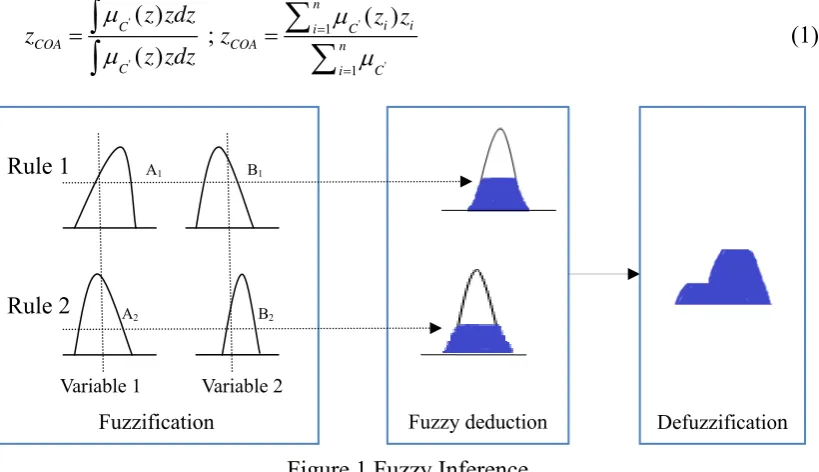
and practicality (Jager, 1995). Figure 1 depicts the min-max fuzzy inference, with two

5

Fuzzy deduction

sets with their respective bell-shaped membership function. In this case, four major

steps should be performed in this fuzzy inference, which are described as follows:

(i) In fuzzifying input variable X1 and X2, the function of antecedence is to

implement the premise part of “if.” The result of “and” or “or” operation _i in the

antecedence represents the degree of fulfillment for the rule i and can be written as:

1 2 1 2

( ) ( ); ( ) ( ) for =1,2

i i i i

i A x B x i A x B x i

     

(ii) The “then” operation is the consequence represented by a fuzzy setC_i in output

variable Z. The fuzzy implication reshapes the consequence with _i given in the

antecedence. The minimum implication is written as:

'( ) ( ) for =1,2

i

i i C

C z z i

  

(iii) The outputs of '( )

i

C z

 for i=1,2 are then aggregated to form a fuzzy setC'in

output variable Z that is written as:

' ' '

1 2

1 2 1 2

( ) [ _C( )] [ _C ( )]

C z C C z z

        

(iv) Finally, the output of aggregation is defuzzified to obtain a crisp output z.

Different methods of defuzzification may be used, such as mean of maximum,

middle of max, center of area (COA), and Center of Gravity. The current paper uses

method of COA to identify the centroid of the fuzzy set. For continuous and

discrete cases, COA is written as:

' ' ' ' 1 1 ( ) ( ) ; ( ) n i i

C i C

COA COA n

C i C

z zdz z z

z z z zdz       









Figure 1 Fuzzy Inference

A1 B1

A2 B2

Variable 1 Variable 2

Fuzzification Defuzzification

6 2.2 Genetic algorithm (GA)

A number of parameters embedded in the fuzzy inference should be determined to

estimate the output variable effectively. For instance, the parameters or shape of the

membership function, which may be Gaussian, trapezoidal, triangular, s-shaped, or

z-shaped function, is a determinant for output estimation. To preclude the excessive

non-linear property, the Gaussian membership function is applied in the present work.

Supposeθis the decision vector to be solved. The optimal problem is to minimize the

objective function of root mean squared error (RMSE) in the fuzzy inference system,

which is written as:

2

1

ˆ ( ) RMSE

n

i i i

z z Min

n

 _







where ˆz_i is the estimation of output z_i for sample I, and n is the sample size.

The rule-based fuzzy inference is non-linear with max-min composition, implying

that the functions in the fuzzy inference are somehow kinked and cannot be

differentiable. Hence, the fuzzy inference system cannot be optimized using the

classical method of direction search. In this complex context, GA based on the

mechanics of natural selection and natural genetics is a better robust algorithm for

implementing the fuzzy optimization. Three major types of operations exist in GA,

namely, selection, reproduction, and mutation, according to the Darwinian evolutionary

theory. For a detailed interpretation and demonstration, a number of previous studies

may be used as reference (Goldberg, 1989; Koza, 1992).

However, the fuzzy inference system has a number of limitations. Aside from its

nonlinear property and inefficiency in computing GA, one major criticism is that the

fuzzy rules are not well developed and cannot be applied to the knowledge-based

system. Thus, to embody the expert knowledge into the fuzzy rules appropriately, the

structural equation modeling, as seen in the next section, is proposed to determine the

concise and integrated structural relationships between input and output variables and

to build the more convincing fuzzy rules as well.

2. 3 Structural equation modeling

The SEM technique enables the examination of complicated phenomena using

hypothetical construct (latent) variables, measurement error, and correlative

7

between variables constructed by the linear relationship is referred to as the SEM

(Tabachnick and Fidell, 1996). The SEM is currently one of the most useful tools for

path analysis in marketing and consumer research (Gefen et al., 2000). SEM is also

frequently used in traveler behavior studies and activity analyses (Kuppam and

Pendyala, 2001).

The SEM group includes “covariance structure analysis,” “latent variable

analysis,” “confirmatory factor analysis,” and the “analysis of linear structural

relationships.” By combining multiple regression and factor analyses, the SEM is

capable of simultaneously analyzing correlations of a group of mutually dependent

variables (Hair, 1998). The SEM functions are essentially used in exploring the

causality between multivariables or univariables that are not supposed to be directly

measured. Although some presumptions have to be made over observed variables and

measurement errors, the unobservable or latent variables are constructed. In the

meantime, the structural model is established between endogenous and exogenous

constructs. Thus, the theoretical structure of SEM comprises the “structural model” and

“measurement model” (Hatcher, 1998). Specifically, the structural model is used to

define the linear relationship between the endogenous and exogenous latent variables,

whereas the measurement model defines the linear relationship between the latent

variables and the observed variables. Thus, the linear relationship developed from the

second model is typically used to extort the observation data before processing the

analysis (Lin, 1984).

3. Data Methods and Description

3.1 Study design

The present study uses the SEM to build an overall Mamdani-type fuzzy influence

system for analyzing reasonable relationships between various observed and latent

variables of the economic index. The observed variables include the USD value, NTD

value, and the USD index, plus the USD/NTD volatility of exchange rate returns that

acts as the risk factor for control. Note that USD/NTD indicates that 1 US dollar is

expressed in New Taiwan Dollars. The output and input variables are converted into

linguistic variables or fuzzy sets using various suitable membership functions. The

major fuzzy rules are then constructed by the SEM of path analysis. To optimize the

fuzzy influence system, the GA is applied to fit the parameters embedded in the

8

constructed to empirically verify the decision of trading.

3.2 Study samples

The study samples are derived from the macroeconomic database of Taiwan

Economic Journal (TEJ) and the Financial Statistics Monthly edited by the Economic

Research Department at the Central Bank of the Republic of China. The study period

covers January 1, 1996 to December 2010, yielding a total of 180 pieces of data that

are regarded as the values of observed variables. To test the robustness of the model,

the data are divided into training period samples and verification period samples. The

training period is from February 1996 to September 2007, whereas the verification

period is from July 2008 to December 2010. Using the available variables, the present

study converts the macroeconomic variables into monthly increase rates for the SEM

rule-based fuzzy model. The measurement scales for different economic indexes vary

widely. Thus, the present study also converts a variety of data into standardized scores

before analyzing or comparing the statistics so as to achieve a good fit between the

model and the data sample.

3.3 Conceptual model construction

According to the theory of SEM and the relevant literature, several variables can

affect the change in exchange rates. The data must be meaningful and informative for

the change in exchange rates. However, including all the variables in the model

construction would be costly and would also make the achievement of the goal difficult.

Thus, although the macroeconomic system widely covers the monetary, financial

securities, and labor markets, the current research followed Walras’ Law by removing

the labor market and selecting five important variables from the remaining three

markets: M2, CPI, GDP, rediscount rate, and stock price index. The present study also

adopted various economic observed values from Taiwan and the US, using these values

for the observed variables that are classified into the 1st and 2nd Groups. The observed

values taken from Taiwan (hereafter referred to as the NTD value) are the endogenous

variables (dependent variables), whereas those from the US (hereafter referred to as the

USD value) are the exogenous variables (independent variables). To better understand

the interaction of economic variables with the exchange rates of the major world

currencies, the present work selects six major international currencies, namely the Euro

(EUR), Japanese Yen (JPY), Great Britain Pound (GBP), Canadian Dollar (CAD),

Swedish Kronor (SEK), and the Swiss Franc (CHF), and attempts to compare the

9

index, the present study computes the values of USD index that are observable and can

be classified as Group 3. The USD index is considered as an endogenous or mediator

variable.

By analyzing foreign exchange related literature, the current research compiles the

data from expert knowledge and infers several hypotheses through the SEM. The

hypotheses include a positive effect of USD value on NTD value and on the USD

index, a positive effect of the USD index on the NTD value, and an indirect effect of

USD value on NTD value through the USD index. The result can be found in Sec. 4.1.

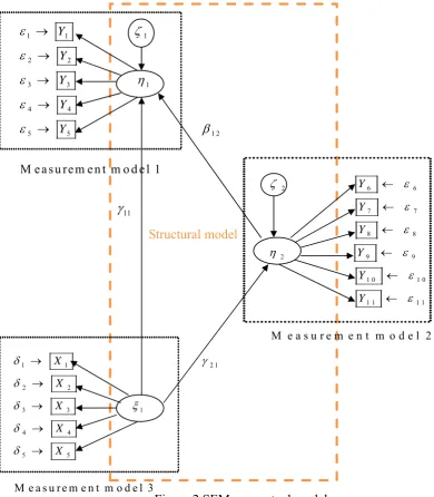
The current research uses the SEM, as shown in Figure 2, to construct the

conceptual model. The measurement and structural models are also built by estimating

the model parameters. The details are shown as follows:

1 1 1

2 2

3 3 1

4 4

5 5 1 2

M e a s u re m e n t m o d e l 1 Y Y Y Y Y              　 11  Structural model

Figure 2 SEM conceptual model

1 1 2 1

2 2

3 3 1

4 4

5 5

M e a s u r e m e n t m o d e l 3

X X X X X             　 　 　 　 　

2 6 6

7 7

8 8

2 9 9

1 0 1 0

1 1 1 1

M e a s u r e m e n t m o d e l 2

10 (1) Measurable equation

(a) Measurement model 1

2 1 11 1 1

2 21 1 2

3 31 1 3

M (NTD Value, measurement error)

CPI (NTD Value, measurement error)

(NTD Value, measurement error)

Re y y y f Y f Y f Y                   TW TW TW GDP

TW _{4 41 1 4}

5 51 1 5

discount rate (NTD Value, measurement error)

Stock price index (NTD Value, measurement error)

y y f Y f Y             TW

(b) Measurement model 2

6 62 2 6

7 72 2 7

8 82 2 8 (US dollar index, measurement error)

(US dollar index, measurement error)

(US dollar index, measurement error)

(US dollar index, me

y y y f Y f Y f Y f                    USD/EUR USD/GBP USD/JPY

USD/CAD _{9 92 2 9}

10 102 2 10

11 112 2 11 asurement error)

(US dollar index, measurement error)

(US dollar index, measurement error)

y y y Y f Y f Y                  USD/CHF USD/SEK

(c) Measurement model 3

2 1 11 1 1

2 21 1 2

3 31 1 3

M (USD Value, measurement error) X

CPI (USD Value, measurement error) X

(USD Value, measurement error) X

Rediscount rate (USD Value, measurement e

x x x f f f f                    US US US GDP

US _{4 41 1 4}

5 51 1 5

rror) X

Stock price index (USD Value, measurement error) X x x f            US

(2) Structural equation

11 12

1 11 1 12 2 1

21

2 21 1 2

NTD = ( USD )+ (US dollar index)+residual error

US dollar index= ( USD )+residual error

                 

Value Value

Value

3.4 SEM structure

The SEM provides an intact comprehensive system for data analysis and

theoretical research. Using SEM, the causality in the structural model and the construct

validity in the measurement model may be simultaneously analyzed and evaluated. The

details of this approach are described below (Hu and Jen, 2008):

11

The structural model shows the causality between a host of latent variables. The

cause-and-effect relationship in the model is generally derived from other theoretical

assumptions. The “cause” assumed in the model is called the exogenous variable,

whereas the “effect” is the endogenous variable. The following shows the structural

model of SEM:

B

      (3)

where  is exogenous variable, is endogenous variable,  stands for the

coefficient matrices of the influence effect of exogenous variables on endogenous

variables, B refers to the coefficient matrices of the influence effect of endogenous

variables on endogenous variables, and  is the vector of the “residual error.”

Three basic hypotheses are given in this model: (i) The variables are represented

by deviation scores, where the average value is 0; (ii) no correlation exists between and ; and (iii) the diagonal line ofBis 0, where IB is a non-singular matrix.

(2) Measurement model

The observed variables use measureable secondary data to observe the effect of

latent variables. The measurement model is used to elaborate on the relationship

between the latent and observed variables.

Generally, the measurement model comprises two equations that define the

association between endogenous latent variables  and endogenous observed

variables y and between exogenous latent variables  and exogenous observed

variablesx. In fact, the measurement model can be considered a measurement and a

kind of reliability description of the observed variables as follows:

y

y    (4)

where y refers to the endogenous observed variables, _y stands for the coefficient

matrices of the relationship between yand, and  is measurement error of y.

x

x    (5)

wherex refers to the exogenous observed variables;_xstands for the coefficient

matrices of the relationship between xand; is measurement error of x; and

y

 and _xare the approximate regression coefficients fory and x, respectively.

12

observed variables can be used to indirectly infer latent variables by assuming the following hypotheses: (i) no correlation exists between the measurement error and,

, or  , but , , and  can be correlated; and (ii) similarly, no correlation exists

between the residual error ( ) and the measurement error (and ).

(3) Inference of covariance matrix

Given SEM’s basic assumptions and under the hypothesis of normal data

distribution, the covariance matrix of Vector z( , )y x  can be theoretically obtained.

The process is described below:

(a) Definition of variables

y

 : p×m coefficient matrix describing the relationship between y and

x

 : q×m coefficient matrix describing the relationship between x and

B : m×m coefficient matrix describing the influence effect ofon itself

Γ: m×n coefficient matrix describing the influence effect ofon

Φ : n×n covariance matrix of

Ψ: m×m covariance matrix of



 : p×p covariance matrix of



 : q×q covariance matrix of

(b) The structural equation model is shown as below:

; _{y x}

B y x

      ;　       

The covariance matrix _xx of exogenous observed variables is obtained as

follows:

( ) ( )

[( )( ) ]

( ) ( ) ( ) ( )

0 0

xx

x x

x x x x

x x

x x

Cov xx E xx E

E E E E





   

   



  



    

   

       



       

    

(6)

13 ( ) ( )

[( )( ) ]

( ) ( ) ( ) ( )

( ) 0 0 yy

y y

y y y y

y y

y y

Cov yy E yy E

E E E E

E _                                                  (7)

The covariance matrix _of endogenous latent variables is obtained as follows:

1 1 1 1

1 1 1 1

1 1 1 1

1 1 ( ) [( ) ( ) ][( ) ( ) ] ( ) ( ) ( ) ( ) ( )( ) ( ) ( ) ( ) ( ) ( ) [ ]( ) E

E I B I B I B I B

I B E I B I B E I B

I B I B I B I B

I B I B

                                                                   (8)

Equation (8) is then substituted into (7) to derive the following:

1 1

[( ) ( )( ) ]

yy y I B I B y 



 _  _

           (9)

The covariance matrix _xyof exogenous observed variables and endogenous observed

variables is obtained as follows:

( ) ( )

[( )( ) ]

( ) ( ) ( ) ( )

( ) 0 0 0 xy

x y

x y x y

x y

x y

Cov xy E xy E

E E E E

E                                                (10)

The covariance matrix _ of endogenous latent variables and exogenous latent

variables is obtained as follows:

1 1 1 1 1 1 ( ) [( ) ( ) ] ( ) ( ) ( ) ( )

( ) 0

( )

E

E I B I B

I B E I B E

I B I B                                    (11) 1

(I B)

  

      , and substituting this formula into Equation (10) yields the

following:

1

(1 )

xy x B y



 _

14

Finally, the covariance matrix is written as yy yx

xy xx

 

 

  _{ } 

 . Combining Equations

(6), (9), and (12) yields the following:

1 1 1

1

[( ) ( )( ) ] (1 )

(1 )

y y y x

x y x x

I B I B B

B







  

 

  

            

   _{       } 

 

  (13)

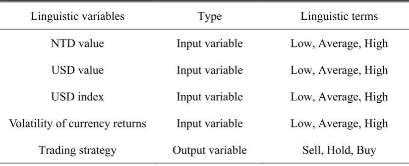
3.5 Linguistic variables and linguistic terms

Table 1 describes the linguistic variables used in the present study, as well as their

linguistic terms. The input linguistic variables are the “NTD value,” the “USD value,”

the “USD index,” and the “Volatility of currency (USD/NTD) returns,” whereas the

output linguistic variable is termed “Trading strategy.” Each linguistic variable has

three linguistic terms, i.e., membership functions.

3.6 The membership function

The membership function describes to what degree of the truth the input variable

represents the membership of vaguely defined sets. The shape of the membership

function can dramatically affect the result of the fuzzy system. The membership

functions are generally determined in accordance with experts’' recommendations and

operation habits. Linear membership functions, including the Gaussian membership

function, are good candidates for use in the fuzzy system. The path analysis derived

through the SEM is significantly more impartial and unprejudiced in operating the

fuzzy sets rationally.

Table 1 Names and types of variables and their linguistic terms

Linguistic variables Type Linguistic terms

NTD value Input variable Low, Average, High

USD value Input variable Low, Average, High

USD index Input variable Low, Average, High

Volatility of currency returns Input variable Low, Average, High

15 3.7 Establishment of fuzzy rules

Fuzzy rules are the most important part of the fuzzy system. Establishing rules

that comply with the status quo requires rule-of-thumb specifications. If the

goodness-of-fit of SEM is inappropriate, the logic of the rules will also be improper.

Hence, determining various rules of thumb is necessary to improve the fuzzy rules.

More reliable decisions can thus be made to achieve better investment performance.

Therefore, based on the rules of thumb inferred from the SEM and the additional rules

involved in the volatility factor, the present study analyzes the fuzzy input variables,

i.e., latent variables and creates 18 fuzzy rules, as shown in Table 2.

3.8 Fuzzy trading system

The present work primarily aims to fuzzify input variables and risks and then use

the GA for fitness so that the relationships between input and output variables could be

more precisely identified. The primary method is to properly convert the four input

variables into the output variable by operating the high, low, or average fuzzy set of

each variable. The numerical values of economic variables are thus transferred into the

linguistic variables of USD and NTD values through the Gaussian membership

functions. Therefore, the fuzzy rules derived from the SEM can be evaluated through

the sample data, and the fuzzy inference system can then be fitted to determine the

parameters embedded in fuzzy sets. A fuzzy trading system is constructed and ready

for verification using the test data.

Table 2 Fuzzy Rules

Rule No. Specification

Rule 01 IF NTD Value High and USD Value High then Strategy is Buy U/N

Rule 02 IF NTD Value low and USD Value low then Strategy is Sell U/N

Rule 03 IF NTD Value average and USD Value average then Strategy is Hold U/N

Rule 04 IF USD Value High and USDX High then Strategy is Buy U/N

Rule 05 IF USD Value low and USDX low then Strategy is Sell U/N

Rule 06 IF USD Value average and USDX average then Strategy is Hold U/N

Rule 07 IF NTD Value High then Strategy is Sell U/N

Rule 08 IF NTD Value low then Strategy is Buy U/N

Rule 09 IF USD Value High then Strategy is Buy U/N

16

Rule 11 IF USDX High then Strategy is Buy U/N

Rule 12 IF USDX low then Strategy is Sell U/N

Rule 13 IF USD Value High and VCR High then Strategy is Buy U/N

Rule 14 IF USD Value low and VCR low then Strategy is Sell U/N

Rule 15 IF USD Value average and VCR average then Strategy is Hold U/N

Rule 16 IF USDX High and VCR High then Strategy is Buy U/N

Rule 17 IF USDX low and VCR low then Strategy is Sell U/N

Rule 18 IF USDX average and VCR average then Strategy is Hold U/N

Notes: 1. “USDX” =USD index. “VCR” =Volatility of currency returns. “Strategy” =Trading strategy.

“U/N” =USD/NTD.

2. Volatility of currency returns is the volatility estimated from GARCH model.

4. Analysis of Empirical Results

4.1 Structural model analysis

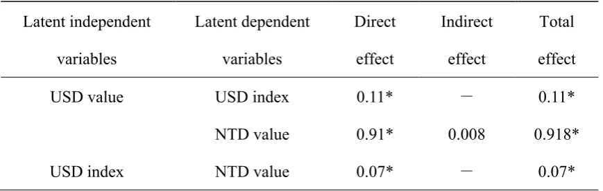
The SEM can be used for path analysis and the decomposition of influence. The

effect of one latent variable on another is called a direct effect, whereas the effect that

occurs from a third latent variable is referred to as an indirect effect. The direct effect

plus the indirect effect is called the total effect. The decomposition chart of the

influence effects is shown in Table 3, and the present study’s overall empirical

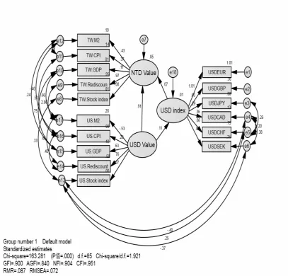
structural model is illustrated in Figure 3.

The model reports that the USD value has a significant effect on the USD and the

NTD value, the USD index has a significant effect on the NTD value and through the

USD index, the USD value has an indirect effect on the NTD value.

Table 3 The Decomposition of the Influence Effects

Latent independent

variables

Latent dependent

variables

Direct

effect

Indirect

effect

Total

effect

USD value USD index 0.11* － 0.11*

NTD value 0.91* 0.008 0.918*

USD index NTD value 0.07* － 0.07*

17

Figure 3 The Overall Empirical Structural Model

4.2 Model fit analysis

According to the evaluation indicators revealed in Figure 3, the Chi-square value

is 163.281, the degree of freedom is 85, and the p-value is 0.000, representing a highly

significant level. The Chi-square value ratio is 1.921 (163.281÷85), which is within the

value of criterion≤3, representing a proper overall fit between the theory model and the

overall observed data.

Moreover, the other goodness-of-fit indices were all found to reach or are

approximate close to the value of the criterion (GFI>0.9; AGFI>0.9; NFI>0.9; CFI>0.9;

RMR<0.08; RMSEA<0.08). This finding illustrates that the overall model of the

18

model based on the SEM factor analysis can appropriately interpret the actual data.

4.3 The buy/sell trading signals

The trading of USD/NTD will give rise to different returns at different times. The

buy-and-sell signals are actually determined by the output variable of the fuzzy

inference system. If the output variable is greater than a specific value, it is viewed as

the buy signal, and if it is smaller than a specific value, it is viewed as the sell signal.

These buy/sell specific points in trading strategy are determined to minimize the error

square between the output variable and the actual exchange rate of return. As a result

of the fuzzy inference trained by the sample data, the buy signal appears when the

output variable exceeds 3.3428, and the sell signal emerges when the output variable is

less than -3.9531.

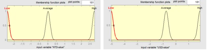
4.4 Membership functions of variables

The membership functions of each variable are obtained with their respective

optimal parameters, which are then fine-tuned by a GA based on the fuzzy rules and

inference in previous section. As a result, Figure 4 exhibits all the empirical

membership functions of the input and output variables.

Figure 4(a) shows the membership functions of the input variable NTD value. The

optimal membership is obtained by genetically searching the parameters with

respective function types (low, average, high) to minimize the objective function of

RMSE, as shown in Equation (2). The results of the optimal membership parameters

for the NTD value are -2.4226 and 2.7706, indicating that when the NTD value is

below -2.4226, a “low value” level is achieved, and when it is above 2.7706, a “high

value” level is reached. Figure 4(b) reveals the membership function of the input

variable USD value. Similarly, the results of the optimal membership parameters for

the USD value are obtained as -5.0779 and 1.8926. A USD value below -5.0779reflects

a “low value” level, whereas a USD value above 1.8926reflects a “high value” level.

Figure 4(c) shows that the optimal membership parameters for the input variable

USDX are -1.4202 and 0.4685, implying that when the USDX is below -1.4202, a “low

index” level is achieved, and when it is above 0.4685, a “high index” level is reached.

Figure 4(d) shows that the optimal membership parameters for the input variable

volatility of currency (USD/NTD) returns are 0.1449 and 0.5461. Hence, when the

volatility of currency returns is below 0.1449, a “low volatility” level is achieved, and

19

that the optimal membership parameters for the trading strategy Sell and Buy are

-3.9531 and 3.3428. A trading strategy value below -3.9531 creates a “Sell USD/NTD”

signal, a value above 3.3428 creates a “Buy USD/NTD” signal, and a value between

-3.9531 and 3.3428generates a “Hold” signal, wherein nothing is available for trading.

The fuzzy GA (FGA) is used to fit the fuzzy model and to optimize the

parameters involved in fuzzy memberships and the fuzzy rules. Figure 5 exhibits the

objective function (fitness) converging stably and smoothly to the best value (around

1800) when the number of generations reaches approximately 40. This finding

indicates that the fuzzy inference system can effectively fit the training samples of

exchange rates through the FGA.

(a) Membership functions of NTD value (b) Membership functions of USD value

(c) Membership functions of USDX (d) Membership functions of VCR

(e) Membership functions of trading strategy

20

0 20 40 60 80 100 120 140 160 180 200

400 600 800 1000 1200 1400 1600 1800

Generations

F

it

nes

s

Best Average Poorest

Figure 5 Convergence of GA

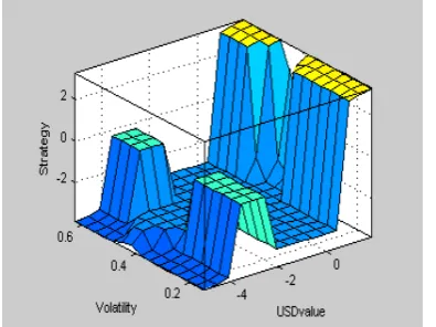
4.5 Changes in input and output variables

Following the training, several three-dimensional charts between the values of

trading strategy versus those of input factors are built according to the optimal fuzzy

rules and inference. The value of trading strategy is apparently noticeable against USD

value and volatility of currency returns or against USDX value and volatility of

currency returns. The results are shown in Figure 6.

(a) Variation in strategy vs. USD value and volatility (b) Variation in strategy vs. USDX and volatility

Figure 6 Variation in trading strategy

Figure 6(a) reveals that the weight of the trading value (importance level) rises as

the volatility or USD value becomes significantly lower or higher. Figure 6(b) shows

that the USD index dominates the volatility in affecting the value of the trading

strategy. However, a comparison of both figures shows that when the USD value or the

USD index is higher, i.e., when the USD/NTD buy point emerges, the effect of

21

importance of volatility risk control for making trading decisions in foreign exchange

markets. Remarkably, when the USD value is lower, thus expressing the sell signal for

USD/NTD trading, the effect of USD value becomes greater.

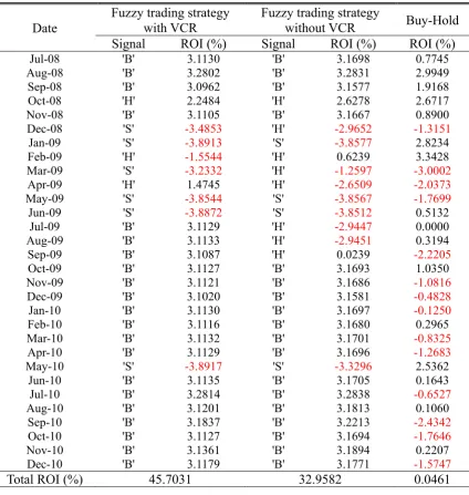
4.6. Investigation of investment performance

The current paper compares the investment performance of the “Fuzzy trading

strategy with Volatility of currency returns,” in which risk is considered, and the

“Fuzzy trading strategy without Volatility of currency returns,” in which risk is

disregarded, as well as the general “Buy-Hold,” i.e., three methods. Table 4 shows the

buy/sell points and return of investment (ROI) rates generated according to the “fuzzy

trading strategy,” in which B represents the “buy signal,” H represents a “hold,” and S

represents the “sell signal.”

The rate of ROI gained from the first operation method is 45.7031%, and that

from the second operation method is 32.9582%, in contrast to merely 0.0461% using

the “Buy-Hold” method. As this comparison emphasizes, applying the “fuzzy trading

strategy” to investments can substantially improve the rate of currency return.

Furthermore, considering the volatility of currency returns can yield better profit than

disregarding such volatility.

5. Conclusion

To construct reasonable fuzzy rules, the present study employed the SEM to

determine the suitable path diagram between various economic indices of observed

variables and their respective latent variables. A risk factor of control, i.e., volatility of

currency returns, was also considered in fuzzy sets. The current research constructed

several fuzzy rules based on SEM path analysis and fitted the parameters of the

memberships of fuzzy sets to the returns of currency data using a GA. According to the

empirical results, the present work has the following conclusions:

(i) Regardless of whether or not the volatility of currency returns is considered,

investments made with the fuzzy trading strategy achieve a significantly better

rate of return than those made using the Buy-Hold method. The returns were

45.7031% and 32.9582% using the two previous methods, whereas a value of

only 0.0461% was obtained using the proposed method.

(ii)Investment using the fuzzy trading strategy, in which the volatility of currency

22 disregarded.

(iii)The trading strategy is apparently affected as the USD value or the volatility

of currency returns shifts into either a higher or lower state.

In summary, the fuzzy trading system has incorporated the SEM path and factor

analyses into fuzzy rules. Moreover, the inclusion of the volatility of currency returns

in the fuzzy trading system certainly helped in acquiring larger excess returns, thus

outperforming the Buy-Hold strategy.

Table 4 Comparison between “Fuzzy trading strategy with Volatility of currency

returns” and “Fuzzy trading strategy without Volatility of currency returns”

and “Buy-Hold”

Date

Fuzzy trading strategy with VCR

Fuzzy trading strategy

without VCR Buy-Hold Signal ROI (%) Signal ROI (%) ROI (%)

Jul-08 'B' 3.1130 'B' 3.1698 0.7745

Aug-08 'B' 3.2802 'B' 3.2831 2.9949

Sep-08 'B' 3.0962 'B' 3.1577 1.9168

Oct-08 'H' 2.2484 'H' 2.6278 2.6717

Nov-08 'B' 3.1105 'B' 3.1667 0.8900

Dec-08 'S' -3.4853 'H' -2.9652 -1.3151

Jan-09 'S' -3.8913 'S' -3.8577 2.8234

Feb-09 'H' -1.5544 'H' 0.6239 3.3428

Mar-09 'S' -3.2332 'H' -1.2597 -3.0002

Apr-09 'H' 1.4745 'H' -2.6509 -2.0373

May-09 'S' -3.8544 'S' -3.8567 -1.7699

Jun-09 'S' -3.8872 'S' -3.8512 0.5132

Jul-09 'B' 3.1129 'H' -2.9447 0.0000

Aug-09 'B' 3.1133 'H' -2.9451 0.3194

Sep-09 'B' 3.1087 'H' 0.0239 -2.2205

Oct-09 'B' 3.1127 'B' 3.1693 1.0350

Nov-09 'B' 3.1121 'B' 3.1686 -1.0816

Dec-09 'B' 3.1020 'B' 3.1581 -0.4828

Jan-10 'B' 3.1130 'B' 3.1697 -0.1250

Feb-10 'B' 3.1116 'B' 3.1680 0.2965

Mar-10 'B' 3.1132 'B' 3.1701 -0.8325

Apr-10 'B' 3.1129 'B' 3.1696 -1.2683

May-10 'S' -3.8917 'S' -3.3296 2.5362

Jun-10 'B' 3.1135 'B' 3.1705 0.1643

Jul-10 'B' 3.2814 'B' 3.2838 -0.6527

Aug-10 'B' 3.1201 'B' 3.1813 0.1060

Sep-10 'B' 3.1837 'B' 3.2213 -2.4342

Oct-10 'B' 3.1127 'B' 3.1694 -1.7646

Nov-10 'B' 3.1361 'B' 3.1894 0.2207

Dec-10 'B' 3.1179 'B' 3.1771 -1.5747

Total ROI (%) 45.7031 32.9582 0.0461

23

References

Anderson, J.C. and D.W. Gerbing, 1988. Structural Equation Modeling in Practice: A

Review and Recommended Two-Step Approach. Psychological Bulletin, 103:3,

411-23.

Bilson, J.F.O., 1981. The Speculative Efficiency Hypothesis. Journal of Business 54,

No.3, 435-451.

Bodnar, G.M., B. Dumas, and R.C. Marston, 2002. Pass-through and exposure. Journal

of Finance 57, 199-232.

Bodnar, G.M. and M.H.F. Wong, 2003. Estimating exchange rate exposures: issues in

model structure. Financial Management 32, 35-67.

Bollen, K.A. and Long, J.S., 1993. Testing Structural Equation Models, Newbury Park

(Ca): Sage.

Branson, W., H. Halttunen, and P. Masson, 1977. Exchange rates in the short run: The

dollar-deutschemark rate. European Economic Review 10, 303-24.

Branson,W.H. and D.W. Henderson, 1985. The Specification and Influence of Asset

Markets. in, Jones, R. W. and P. B. Kenen,(ed.). Handbook of International

Economics. Volume, North Holland. Amsterdam.

Chan, K.C.C., Lee, V., Leung, H, 1997. Generating fuzzy rules for target tracking using

a steady-state genetic algorithm. IEEE Trans. Evolutionary Computation, 189-200.

Doidge, C., Griffin, J. and Williamson, R., 2006. Measuring the economic importance

of exchange rate exposure? Journal of Empirical Finance 13, 550-576.

Eichengreen, Barry, and Raul Razo-Garcia, 2006. The International Monetary System

in the Last and Next 20 Years. Economic Policy Vol. 21(47), 393–442.

Frenkel, J.A., 1981. Flexible Exchange Rates, Prices, and the Role of “News”: Lessons

from the 1970s＂. Journal of political Economic Vol.54, 665-703.

Gefen, D., D.W. Straub, and M-C Boudreau, 2000. Structural Equation Modeling and

Regression: Guidelines for Research Practice. Communications of the Association

for Information Systems Vol. 4, Article 7.

Goldberg, D.E., 1989. Genetic algorithms in search optimization and machine learning.

Reading. MA: Addison-Wesley Publishing Company, 412.

Hair, J.F., R.E. Anderson, R.L. Tatham, W.C. Black, 1998. Multivariate Data Analysis.

Prentice Hall.

24

Analysis and Structural Equation Modeling. SAS Institute Inc.

Hu, K.C. and Jen W., 2008. Exploring the Effects of Relational Performance and

Service Quality on Customer's Satisfaction and Loyalty in the Freight Shipping

Industry from the Viewpoint of Business-to-Business. Journal of the Chinese

Institute of Transportation 20.2, 201-228.

Jöreskog, K.G., 1973. A general method for estimating a linear structural equation

system. In Goldberger, A. S., & Duncan, O. D. (Eds). Structural Models in the

Social Science. New York: Academic Press.

Jöreskog, K.G. and D. Sörborn, 1996. LISREL 8: user’s reference guide. Scientific

Software International, Chicago.

Jager, R, 1995. Fuzzy Logic in Control. Delft TU Publisher. Delft. The Netherlands.

Karr, C.L., 1991. Genetic algorithms for fuzzy controllers. AI Expert 6(2), 27 -33.

Karr, C.L., 1993. Fuzzy control of pH using genetic algorithms. IEEE Trans Fuzzy

Syst 1, 46 –53.

Koedijk, K.G., Kool, C.J.M., Schotman, P.C., and Dijk, M.A.van, 2002. The cost of

capital in international financial markets: local or global? Journal of International

Money and Finance 21, 905-929.

Kuppam, A.R. and Pendyala, R.M., 2001. A Structural Equations Analysis of

Commuter Activity and Travel Patterns. Transportation 28(1), 33-54.

Lin, C.H., 1984. Theories and Applications of Structural Equation Models and

LISREL IV Program. Psychological Testing 31, 149-163.

Mamdani, E. and S. Assilian, 1975. An experiment in linguistic synthesis with fuzzy

logic controller. Journal of Man–Machine Studies 7(1), 1-13.

Mamdani, E., 1976. Advances in the linguistic synthesis of fuzzy controllers. Journal

of Man–Machine Studies 8, 669-678.

Moffet, M. and J. Karlsen, 1994. Managing foreign exchange rate economic exposure.

Journal of International Financial Management and Accounting 5. 2, 157-175.

Neely, C.J., 2005. An Analysis of Recent Studies of the Effect of Foreign Exchange

Intervention. Federal Reserve Bank of St. Louis Review Nov./Dec.87(6), 685-717.

Tabachnick, B.G. and L.S. Fidell, 1996. Using multivariate statistics (3rd) NY: Harper

Collins.

Williamson, R., 2001. Exchange rate exposure and competition: evidence from the

automotive industry. Journal of Financial Economics 59, 441-475.

25

Zadeh, L.A., 1996. Fuzzy sets, fuzzy logic, and fuzzy systems: selected papers:

Advances in fuzzy systems-applications and Theory.vol. 6. NJ: World Scientific.

Zimmermann, H.J., 1996. Fuzzy Sets Theory and its Applications, third ed. Kluwer