Numerical Solution of Klein/Sine Gordon Equations by Spectral Method Coupled with Chebyshev Wavelets

(1)

http://www.scirp.org/journal/am ISSN Online: 2152-7393 ISSN Print: 2152-7385

Numerical Solution of Klein/Sine-Gordon

Equations by Spectral Method Coupled with

Chebyshev Wavelets

Javid Iqbal, Rustam Abass

Department of Mathematical Sciences, BGSB University, Rajouri, India

Abstract

The basic aim of this paper is to introduce and describe an efficient numerical scheme based on spectral approach coupled with Chebyshev wavelets for the ap-proximate solutions of Klein-Gordon and Sine-Gordon equations. The main charac-teristic is that, it converts the given problem into a system of algebraic equations that can be solved easily with any of the usual methods. To show the accuracy and the ef-ficiency of the method, several benchmark problems are implemented and the com-parisons are given with other methods existing in the recent literature. The results of numerical tests confirm that the proposed method is superior to other existing ones and is highly accurate.

Keywords

Chebyshev Wavelets, Spectral Method, Operational Matrix of Derivative, Klein and Sine-Gordon Equations, Numerical Simulation, MATLAB

1. Introduction

Many physical phenomena encountered in science and engineering are governed by ordinary as well as partial differential equations. Some disciplines that use partial differential equations to describe the phenomena of interest are fluid mechanics, solid mechanics, quantum mechanic, propagation of acoustic and electromagnetic waves and problems in heat and mass transfer. Many linear and nonlinear phenomena appear in several areas of scientific fields like physics, chemistry and biology can be modeled by different type of partial differential equation such as evolution equation, reaction diffu- sion equation, Schrodinger type wave equations, Vander Poll’s equation, Telegraph equation, Lyapunov equation etc. A broad class of analytical methods and numerical

How to cite this paper: Iqbal, J. and Abass, R. (2016) Numerical Solution of Klein/Sine- Gordon Equations by Spectral Method Coupled with Chebyshev Wavelets. Applied Mathe-matics, 7, 2097-2109.

http://dx.doi.org/10.4236/am.2016.717167 Received: September 5, 2016

Accepted: November 12, 2016 Published: November 15, 2016 Copyright © 2016 by authors and Scientific Research Publishing Inc. This work is licensed under the Creative Commons Attribution International License (CC BY 4.0).

http://creativecommons.org/licenses/by/4.0/

(2)

methods available in the literature are used to handle these problems. In this present work we are dealing with two partial differential equation named as Klein-Gordon and Sine-Gordon equations. The Klein-Gordon equation is as follows:

( )

(

,

) (

, ,

)

, 0

tt xx yy

u −αu −βu +g u = f x y x y ∈ Ω ≥t (1)

where u=u x t

( )

, represents the wave displacement at position x and time t, α and

β are known constant, g u

( )

is the given nonlinear force and f is the known

function. If we assign the nonlinear force g u

( )

=sinu in (1) then it is known as Sine-

Gordon equation. The Klein-Gordon equation plays an important role in mathematical

physics [1] [2] [3] and attracted more attention from scientists and engineering in

different matter like investigation of the interaction of solutions in a collisionless plasma, the recurrence of initial states and examination of the nonlinear wave equations, studying the solutions and condensed matter physics and relativistic physics as a model of dispersive phenomena. On the other hand, Sine-Gordon equations appeared in many physical problems like applications in relativistic field theory, Josephson junc-

tions or mechanical transmission lines [4] [5] [6] [7]. Numerical solution of partial

differential equations is far more demanding than the ordinary ones. Several analytical

or numerical methods such as decomposition method [8], variational iteration method

[9], He’s variational iteration method [10], collocation and radial basis functions [11],

auxiliary equation method [12], spectral method [13] [14] [15], wavelet method [16]

[17][18] and the references therein have been proposed for the numerical solution of

these types of equations. Among all these method mentioned above, spectral and wavelet method has got more attention of researcher from the last two decades.

Wavelet analysis had made a lot of successes in different fields of science and engi-neering due to its beautiful properties such as orthogonality, multi-resolution analysis and computational efficiency. Wavelet permits the accurate representation of a variety of functions and operators. Wavelet analysis and wavelet transform are recently devel-oped mathematical tool for solving the linear and non-linear ordinary differential equa-tions, partial differential equations and integral equation. Wavelets also applied in nu-merous disciplines such as image compression, data compression and deionising data. Most commonly wavelets are Haar, Legendre, Chebyshev are used to find the numeri-cal solution of partial differential equations. In addition wavelet approach can make a connection with some fast and reliable numerical methods. The spectral method has the advantage of exponential convergence property when orthogonal basis functions are involved. As a result, it plays a vital role in solving partial differential equation. It is important to choose the basis function for possible coupling with spectral method. The wavelet basis can combine the advantages of both infinitely differentiable and small compact support which is far better than the spectral and finite element basis.

In recent year, spectral method [19][20] using Legendre polynomials and Legendre

wavelets as basic functions are considered to solve the Klein-Gordon and Sine-Gordon

equations. By inspiring the work done in [19] [20], we use the Chebyshev wavelet as

(3)

wavelet basis can obtain good spatial and spectral resolution while still keeping high ef-ficiency.

The rest of the paper is as follows: In Section 2, Chebyshev wavelet and its properties are discussed. Operational matrix of derivative required for our subsequent develop-ment is presented in Section 3. Section 4 is devoted to present the Chebyshev wavelets spectral collocation method for solving Klein-Gordon and Sine-Gordon equations then approximate the unknown function. Section 5 deals with the illustrative examples and their solutions by the proposed approach compared with exact as well as with existing literature. Finally, concluding remarks are made in Section 6.

2. Wavelets and Chebyshev Wavelets

In the past decades, wavelets [21] [22] [23] shows their interest in different fields of

science and technology due to its beautiful properties. Wavelets constitute the family of functions constructed from the dilation and translation of a single function known as the Mother wavelet. When the dilation parameter a and translation parameter b vary

continuously we have the following family of continuous wavelets [23]

( )

1 2

, ; , , 0.

a b t

t b

a a b a

a

ψ − ψ − 

= _ _ ∈ ≠

   (2)

If we choose 0

k

a=a− and b=nb a₀ −k where a₀ >1,b₀ >0 and n k, ∈+ then we

get the following family of discrete wavelets:

( )

2

(

)

, 0 0 0 .

k k

k n t a a t nb

ψ ₌ − ψ ₋

(3)

These family of functions are a wavelet basis for 2

( )

L  and makes an orthonormal

basis for the special case a0=2 and b0=1.

Chebyshev wavelets ψn m,

( )

t =ψ

(

k m n t, , ,

)

have four arguments, k=0,1, 2,,

1, 2, , 2k

n=  , m is the degree of Chebyshev polynomial of first kind and t denotes the

normalized time. They are defined on the interval

[

0,1

)

by

( )

(

)

2 1

,

2 1

2 2 1 ,

2 2

π

0, otherwise k

k m

m k k

n m

n n

T t n t

t

α

ψ +

 −

− + ≤ ≤

 =   

(4)

where

2, 0

2, 1, 2, m

m m

α =  =

=

 

( )

m

T t in (4) are well known Chebyshev polynomial of order m, which is orthogonal

with respect to the weight function

( )

1 ₂

1 t

t

ω =

− and satisfy the following recursive

formula:

( )

0 1

T t =

( )

1

(4)

( )

1 2 1 , 1, 2, 3, .

m m m

T ₊ t = tT t −T ₋ t m= 

Moreover, the set of Chebyshev wavelet are an orthogonal set with respect to the

weight function

( )

(

1

)

2k 2 1

n t t n

ω ₌ω + ₋ ₊ _.

Any function

( )

2

[ ]

0,1

f t ∈L may be expanded in terms of Chebyshev wavelet as

( )

1 0

, nm nm n m

f t c ψ t

∞ ∞

= =

=

∑∑

(5)

where the wavelet coefficients of the series representation in (5) become

( )

,

( )

_{( )}.

n

nm nm _{w t}

c = f t ψ t (6)

If the infinite series in (5) is truncated then Equation (5) can be written as

( )

2 1 1

( )

T

( )

1 0

,

k _M

nm nm n m

f t c ψ t C t

− ₋

= =

≅

∑ ∑

= Ψ ₍₇₎

where C and Ψ

( )

t are 1

2k 1 M

− _× _{matrices given by:}

1 1

T

1,0, 1,1, , 1,M1, 2,0, 2,1, , 2,M 1, , ₂k _,0, , ₂k _M ₁ ,

C= c c  c − c c  c −  c −  c − ₋_ (8)

( )

1 1

T

1,0, 1,1, , 1,M1, 2,0, 2,1, , 2,M 1, , 2k ,0, , 2k ,M1 .

t ψ ψ ψ − ψ ψ ψ − ψ − ψ − ₋

Ψ _{= }     _ (9)

3. Chebyshev Wavelets Operational Matrix of Derivative

In this section, we first derive the operational matrix D of derivative which plays a great role in order to reducing the given problem into solving the system of algebraic equation. For this, we concern with some Theorem and Corollary as follows.

Theorem 1 [24]. Let Ψ

( )

t be the Chebyshev wavelets vector defined in (9), then we

have

( )

_{( )}

d

, d

t

D t

t Ψ

= Ψ (10)

where D is 2k

(

_M+1

)

_{operational matrix of derivative as follows:}

,

F O O

O F O

D

O O F

…

 

 _… 

 

=

 

 _… 

 

    (11)

in which O is an

(

M − ×1

) (

M +1

)

zero matrix, F is an

(

M+1

)(

M +1

)

matrix and

its

( )

i j th, element is defined as follows:

(

)(

)

(

)

(

)

1 ,

2 2 1 2 1 , 2, , 1 , 1, , 1 and is odd

0, otherwise. k

i j

r s i M j i i j F

+

 ₋ ₋ ₌ ₊ ₌ ₋ ₊

 =  

  ₍₁₂₎

Corollary 1. By using Equation (10), the operational matrix for nth derivative can be derived as

( )

_{( )}

d

, d

n

n n

t

D t

t Ψ

(5)

where n

D is the nth power of matrix D.

4. Chebyshev Wavelets Spectral Collocation Method

In different type of numerical methods, spectral methods are one of the most popular methods of discretization for the numerical solution of partial differential equations and integral equations. The main advantage of this method lies in their accuracy for a given number of unknowns. For smooth problems in simple geometries, they offer ex-ponential rates of convergence or spectral accuracy. In the recent literature, Galerkin, collocation, and Tau methods are the three most widely used spectral versions, in which collocation methods have become increasingly popular for solving differential equa-tions, also they are very useful in providing highly accurate solutions to nonlinear dif-ferential equations. Now, we focus on the solution nature of this method as follows:

Let us consider the equation in the form:

( )

, ,

[

,

]

, 0,

tt xx L R

u −αu +g u = f x t x∈ x x t≥ (13)

with the initial conditions

( )

, 0 1

( )

,

( )

, 0 2

( )

, , 0

u x g x u x g x x t

t ∂

= = ∈ Ω ≥

∂ (14)

or boundary conditions

( ) ( )

, , , , 0.

u x t =h x t x∈ ∂Ω >t (15)

In order to transform the arbitrary domain xL ≤ ≤x xR into the domain defined for

Chebyshev wavelet basis 0≤ ≤x 1, on can use the translation

[

] [ ]

( )

: , 0,1 , L

L R

R L

x x x x x X x

x x

−

→ =

−

By employing θ_{-weight scheme}_[20]_{, discreting the Equation (13), we can get}

( )

(

)

( )

1 1 2 1 2

2 2 2

2

1 , 0 1,

n n n n n

n n

u u u u u

g u f

x x

t θ α θ α θ

+ ₋ ₊ − _ _∂ + _ _ _∂ _

= _ _− − _ _+ = < ≤

∂ ∂

∆     (16)

where ∆t is the time step size with the expression un

( )

x =u t x

(

n,

)

,tn= × ∆n t.

Now Equation (16) becomes

( )

(

)( )

( )

2 1 2

1

2

2 2 2 1

2

2 1 .

n n

n

n n n n

u u t

x u

u t t g u t f u x

θ α

θ

+ +

−

 ∂ 

− _{∆ } _

∂

 

∂ 

= + − ∆ _ _− ∆ + ∆ −

∂

 

(17)

In the light of Equation (7),the term n

u can be expanded by Chebyshev wavelet as

( )

T

( )

. n

n

u x =C Ψ x (18)

Submitting Equation (18) into Equation (17), we have

( )

(

)

( ) ( )

2

(

( )

)

( )

2

T T T T

1 1 ,

n

n L n R n n

C₊Hψ x = C H −C₋ ψ x − ∆t g C ψ x + ∆t f (19)

in which

( )

2 ₂

L

H = −I αθ ∆t D and

(

)( )

2 2

2 1

R

(6)

vative matrix taken from Equation (10)

Also, by using the boundary conditions given in Equation (15), one can get

( )

(

)

( )

(

)

T T

1 0 0, 1 and 1 1 1, 1 .

n n n n

C+Ψ =h t + C +Ψ =h t + (20)

Collocating Equation (19) in ₂k−1_M−₂ Gauss-Chebyshev points

{ }

2 1 1

2

k _M

i i x

− ₋

= , we

have

( )

(

)

( ) ( )

2

(

( )

)

( )

2

(

)

T T T T

1 1 , .

n

n L i n R n i n i i n

C₊H Ψ x = C H −C₋ Ψ x − ∆t g C Ψ x + ∆t f x t (21)

Equation (20) and (21) can be written as matrix form

1 ,

n

AC+ =B (22)

where A and B are 1 1

2k− M×2k− M and 2k−1M×1 matrices, respectively.

Again using the first and second initial conditions given in Equation (14), we have

( )

T

0 i ,

C Ψ x =g x x∈ Ω (23)

and

( )

1 1

2 ,

2

u u

g t x t

− −

= ∈ Ω

∆ (24)

Equation (24) can be written as

( )

T T

1 1 2 2

C−Ψ x =C Ψ x − ∆tg x

Equation (22) using Equation (23) gives a linear system of equations with 1

2k− M

unknown and equations, which can be solved to find Cn+1 in each step n=0,1, 2,

so the unknown function u x t

(

, _n

)

in any time t=t_n can be found. Moreover, we

defined the error bound for

2

L

e and e_L

∞ as

( )

2

1

, max ,

M

j j

L L _j

j

e e e e

∞

=

∑

=

where ej =

(

uexact

)

j−

(

uapprox

)

j and e=uexact−uapprox.

5. Numerical Results and Discussions

In this section, we use Chebyshev wavelets spectral collocation method described in section 4 to solve nonlinear type of Klein-Gordon and Sine-Gordon equations. The proposed method provides a reliable technique which is computer oriented if compared with traditional techniques. To give the clear overview of this method we consider three examples of Klein-Gordon equation and Sine-Gordon equation. All the results are calculated by using the symbolic calculus software MATLAB 2013a and Mathematica.

Example 1 [25] We consider the nonlinear Klein-Gordon Equation (13) with α =1,

( )

2

g u =u and f x t

( )

, = −xcost+x2cos2t in the interval

[

−1,1

]

with the initial

conditions

( )

, 0 , , 0t

( )

0, 1 1

u x =x u x = − ≤ ≤x

and the Dirichlet boundary condition

( ) ( )

, , , , 0.

(7)

The analytical solution is given by

( )

, cos . f x t = −x t

The obtained L2 and L∞ errors of Example 1 at step size 0.0001 is presented in

comparison with the existing method in Table 1 and Table 2 for k=2,M =3 and

2, 4

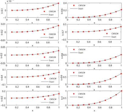
[image:7.595.40.556.236.453.2]

k= M= and graphically shown in Figure 1 for k=2,M =4. It is evident from

Table 1, Table 2 and Figure 1 that the solutions obtain by using CWSCM are in good

agreement and are better than the results obtained by existing method presented in [25].

However, the errors may be reduced significantly if we increase level of resolution.

Table 1. L2 and L∞ error of Example 1 at k=2,M =3 and compared with [25].

( )

2 3

L M= L∞(M=3)

t CWSCM MFDCM [25] CM [25] CWSCM MFDCM [25] CM [25]

0.1 14

3.1 10× − 12

2.2 10× − 4

1.7 10× − 12

5.3 10× − 12

3.5 10× − 4

2.6 10× −

0.2 14

6.4 10× − 12

8.2 10× − 4

4.4 10× − 12

4.8 10× − 11

1.3 10× − 4

3.5 10× −

0.3 12

4.0 10× − 11

1.7 10× − 4

3.6 10× − 12

6.0 10× − 11

2.5 10× − 4

2.3 10× −

0.4 13

1.4 10× − 11

2.7 10× − 4

4.0 10× − 12

4.1 10× − 11

4.1 10× − 4

3.1 10× −

0.5 13

9.6 10× − 11

3.7 10× − 4

4.2 10× − 12

7.5 10× − 11

5.7 10× − 4

3.3 10× −

0.6 13

3.5 10× − 11

4.7 10× − 4

3.5 10× − 12

8.9 10× − 11

6.9 10× − 4

2.6 10× −

0.7 13

2.9 10× − 11

5.5 10× − 4

3.8 10× − 12

2.0 10× − 11

6.8 10× − 4

2.4 10× −

0.8 13

5.7 10× − 11

6.0 10× − 4

2.9 10× − 12

5.4 10× − 11

8.2 10× − 4

3.0 10× −

0.9 13

3.7 10× − 11

6.2 10× − 4

2.7 10× − 12

7.3 10× − 11

8.1 10× − 4

2.5 10× −

1.0 12

8.3 10× − 11

5.9 10× − 4

2.3 10× − 11

5.2 10× − 11

8.1 10× − 4

[image:7.595.43.555.486.707.2]

2.2 10× −

( )

2 4

L M= L∞(M =4)

0.1 14

6.4 10× − 14

5.6 10× − 5

4.1 10× − 13

5.3 10× − 14

6.7 10× − 5

6.7 10× −

0.2 14

5.5 10× − 13

9.6 10× − 5

3.6 10× − 14

1.3 10× − 12

4.1 10× − 5

4.2 10× −

0.3 13

5.4 10× − 12

2.4 10× − 5

4.9 10× − 13

9.1 10× − 12

3.8 10× − 5

5.6 10× −

0.4 13

7.9 10× − 12

4.7 10× − 5

5.4 10× − 13

7.5 10× − 12

5.9 10× − 5

7.3 10× −

0.5 13

8.1 10× − 12

4.2 10× − 5

6.3 10× − 13

6.9 10× − 12

5.8 10× − 5

8.3 10× −

0.6 13

4.5 10× − 12

4.8 10× − 5

4.5 10× − 13

1.4 10× − 12

7.3 10× − 5

6.6 10× −

0.7 13

4.7 10× − 12

6.3 10× − 5

5.8 10× − 13

6.2 10× − 12

8.2 10× − 5

7.4 10× −

0.8 13

7.3 10× − 12

7.1 10× − 5

7.0 10× − 13

8.9 10× − 12

8.9 10× − 5

8.1 10× −

0.9 13

9.4 10× − 12

6.9 10× − 5

5.2 10× − 13

9.7 10× − 12

8.8 10× − 5

7.9 10× −

1.0 13

9.6 10× − 12

6.4 10× − 5

5.3 10× − 13

4.1 10× − 12

8.7 10× − 5

(8)

[image:8.595.51.550.67.442.2]

Figure 1. Comparison of exact solution with approximate solution for Example 1 at k=2,M =4.

Example 2 [25] We consider the nonlinear Klein-Gordon Equation (13) with α =1,

( )

2

g u =u and

( )

(

2 2

)

6 6

, 6

f x t = xt x −t +x t in the interval

[ ]

0,1 with the initial con-

ditions

( )

, 0 0, , 0_t

( )

0, 0 1

u x = u x = ≤ ≤x

and the Dirichlet boundary condition

( )

,

( )

, , , 0.

u x t =h x t x∈ ∂Ω >t

The analytical solution is given by

( )

3 3

, .

f x t =x t

The L2 and L∞ errors of Example 2 at step size 0.0001 are presented in com-

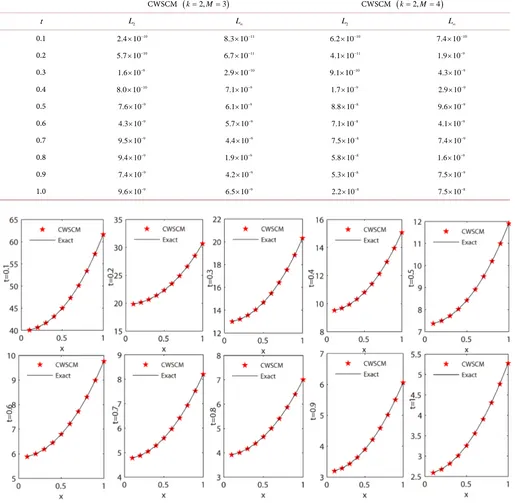
parison with the existing method in Table 3 and Table 4 for k=2,M =3 and k=2,

4

M = . From Table 3, Table 4 and Figure 2, it is clear that CWSCM performs much

better than existing methods [25] and with the increase in number of collocation points

(9)

[image:9.595.43.559.93.296.2]

( )

2 3

L M= L∞(M =3)

0.1 11

4.5 10× − 9

3.9 10× − 4

1.5 10× − 12

1.5 10× − 9

6.0 10× − 4

3.1 10× −

0.2 11

6.5 10× − 8

6.3 10× − 4

1.7 10× − 12

7.3 10× − 8

9.2 10× − 4

3.5 10× −

0.3 10

3.4 10× − 7

3.0 10× − 4

9.7 10× − 12

7.2 10× − 7

4.7 10× − 4

1.8 10× −

0.4 10

5.9 10× − 7

9.1 10× − 4

1.8 10× − 12

6.4 10× − 6

1.4 10× − 4

3.7 10× −

0.5 11

9.3 10× − 6

1.2 10× − 4

9.7 10× − 12

1.9 10× − 6

3.0 10× − 4

2.5 10× −

0.6 10

2.6 10× − 6

4.2 10× − 4

1.7 10× − 12

1.4 10× − 6

5.8 10× − 4

3.7 10× −

0.7 10

1.7 10× − 6

3.2 10× − 4

1.6 10× − 12

2.8 10× − 6

5.9 10× − 4

3.6 10× −

0.8 10

3.6 10× − 6

6.1 10× − 4

1.1 10× − 12

7.3 10× − 6

7.3 10× − 4

2.2 10× −

0.9 10

5.4 10× − 6

5.7 10× − 4

2.0 10× − 12

9.4 10× − 6

6.8 10× − 4

4.5 10× −

1.0 10

1.4 10× − 6

5.5 10× − 4

8.7 10× − 11

6.1 10× − 6

7.5 10× − 4

2.4 10× −

( )

2 4

L M= L∞(M =4)

0.1 11

1.9 10× − 10

4.4 10× − 5

3.6 10× − 11

3.2 10× − 10

5.3 10× − 5

5.3 10× − 0.2 10

4.3 10× − 9

7.8 10× − 5

3.9 10× − 11

5.1 10× − 9

9.4 10× − 5

5.7 10× − 0.3 9

7.1 10× − 8

4.5 10× − 5

2.7 10× − 11

9.0 10× − 8

5.5 10× − 5

4.1 10× − 0.4 9

9.4 10× − 7

1.7 10× − 5

3.8 10× − 10

1.3 10× − 7

3.8 10× − 5

5.6 10× − 0.5 9

6.0 10× − 7

3.1 10× − 5

3.2 10× − 9

2.8 10× − 7

5.6 10× − 5

4.5 10× − 0.6 9

5.3 10× − 7

5.6 10× − 5

3.4 10× − 9

7.9 10× − 7

7.1 10× − 5

5.9 10× − 0.7 9

9.1 10× − 7

5.4 10× − 5

3.5 10× − 9

6.5 10× − 7

7.0 10× − 5

5.9 10× − 0.8 9

6.4 10× − 7

6.8 10× − 5

3.1 10× − 9

5.2 10× − 7

8.6 10× − 5

4.5 10× − 0.9 9

7.1 10× − 7

7.2 10× − 5

3.8 10× − 9

8.4 10× − 7

7.9 10× − 5

6.3 10× − 1.0 9

4.6 10× − 7

6.0 10× − 5

3.3 10× − 9

1.0 10× − 7

8.2 10× − 5

4.6 10× −

Example 3 [20] Consider the following nonlinear Sine-Gordon equation

2 2

2 2 sin 0, 10 10, 0

u u

u x t

t x

∂ ∂

− + = − ≤ ≤ >

∂ ∂

where f x t

( )

, =0, and the initial conditions

( )

, 0 0, _t

( )

, 0 4sech

( )

, 0 1

u x = u x = x ≤ ≤x

and the Dirchlet boundary conditions

( )

,

( )

, , , 0.

u x t =h x t x∈ ∂Ω ≥t

The exact solution is given by

( )

1

(

( )

)

, 4 tan sech

[image:9.595.43.554.329.526.2]

(10)

[image:10.595.150.555.75.443.2]

Figure 2. Comparison of exact solution with approximate solution for Example 2 at k=2,M=4.

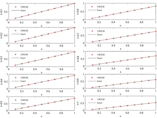
The numerical solution of Sine-Gordon equation has presented in Table 5 which

shows the comparison of the errors of the present method with the exact solution. It is obvious from the table that the present method is more accurate, simple and fast.

Comparison between an exact and approximate solution is shown in Figure 3.

6. Concluding Remarks

(11)

[image:11.595.43.558.96.599.2]

Table 5. L2 and L∞ error of Example 3 at k=2,M =3 and 4.

CWSCM (k=2,M=3) CWSCM (k=2,M=4)

t L2 L∞ L2 L∞

0.1 10

2.4 10× − 11

8.3 10× − 10

6.2 10× − 10

7.4 10× −

0.2 10

5.7 10× − 11

6.7 10× − 11

4.1 10× − 9

1.9 10× −

0.3 9

1.6 10× − 10

2.9 10× − 10

9.1 10× − 9

4.3 10× −

0.4 10

8.0 10× − 9

7.1 10× − 9

1.7 10× − 9

2.9 10× −

0.5 9

7.6 10× − 9

6.1 10× − 8

8.8 10× − 9

9.6 10× −

0.6 9

4.3 10× − 9

5.7 10× − 8

7.1 10× − 9

4.1 10× −

0.7 9

9.5 10× − 9

4.4 10× − 8

7.5 10× − 9

7.4 10× −

0.8 9

9.4 10× − 9

1.9 10× − 8

5.8 10× − 9

1.6 10× −

0.9 9

7.4 10× − 9

4.2 10× − 8

5.3 10× − 9

7.5 10× −

1.0 9

9.6 10× − 9

6.5 10× − 8

2.2 10× − 8

7.5 10× −

Figure 3. Comparison of exact solution with approximate solution for Example 3 at k=2,M =4.

Acknowledgements

We thank the Editor and the referee for their comments.

References

(12)

Equation Using Radial Basis Functions. Journal of Computational and Applied Mathemat-ics, 230, 400-410. http://dx.doi.org/10.1016/j.cam.2008.12.011

[2] Dehghan, M., Mohebbi, A. and Asghari, Z. (2009) Fourth-Order Compact Solution of the Nonlinear Kleingordon Equation. Numerical Algorithms, 52, 523-540.

http://dx.doi.org/10.1007/s11075-009-9296-x

[3] Wazwaz, A.M. (2005) The Tanh and the Sine-Cosine Methods for Compact and Noncom-pact Solutions of the Nonlinear Klein-Gordon Equation. Applied Mathematics and

Com-putation, 167, 1179-1195. http://dx.doi.org/10.1016/j.amc.2004.08.006

[4] Duncan, D.B. (1997) Symplectic Finite Difference Approximations of the Nonlinear Klein- Gordon Equation. SIAM Journal on Numerical Analysis, 34, 1742-1760.

http://dx.doi.org/10.1137/S0036142993243106

[5] Grella, G. and Marinaro, M. (1978) Special Solutions of the Sine-Gordon Equation in 2 + 1 Dimensions. Lettere al Nuovo Cimento, 23, 459-464. http://dx.doi.org/10.1007/BF02770537

[6] Koshelev, A.E. (2010) Stability of Dynamic Coherent States in Intrinsic Josephson-Junction Stacks near Internal Cavity Resonance. Physical Review B, 82, 174-512.

http://dx.doi.org/10.1103/PhysRevB.82.174512

[7] Krasnov, V.M. (2010) The Emission form Intrinsic Josephson Junctions at Zeros Magnetic Field via Breather Auto-Oscillations. Physical Review B, 83, 174-512.

[8] El-Sayed, S.M. (2003) The Decomposition Method for Studying the Klein-Gordon Equa-tion. Chaos Solitons & Fractals, 18, 1025-1030.

http://dx.doi.org/10.1016/S0960-0779(02)00647-1

[9] Batiha, B., Noorani, M.S.M. and Hashim, I. (2007) Numerical Solution of Sine-Gordon Eq-uation by Variational Iteration Method. Physics Letters A, 370, 437-440.

http://dx.doi.org/10.1016/j.physleta.2007.05.087

[10] Shakeri, F. and Dehghan, M. (2008) Numerical Solution of the Klein Gordon Equation via He’s Variational Iteration Method. Nonlinear Dynamics, 51, 89-97.

http://dx.doi.org/10.1007/s11071-006-9194-x

[11] Dehghan, M. and Shokri, A. (2008) A Numerical Method for One-Dimensional Nonlinear Sine-Gordon Equation Using Collocation and Radial Basis Functions. Numerical Methods

for Partial Differential Equations, 24, 687-698. http://dx.doi.org/10.1002/num.20289

[12] Sirendaoreji (2007) Auxiliary Equation Method and New Solutions of Klein-Gordon Equa-tions. Chaos, Solitons & Fractals, 31, 943-950. http://dx.doi.org/10.1016/j.chaos.2005.10.048

[13] Guo, B.-Y., Xun, L. and Vazquez, L. (1996) A Legendre Spectral Method for Solving the Nonlinear Klein-Gordon Equation. The Journal of Computational and Applied Mathemat-ics, 15, 19-36.

[14] Li, X. and Guo, B. Y. (1997) A Legendre Spectral Method for Solving the Nonlinear Klein- Gordon Equation. Journal of Computational Mathematics, 15, 105-126.

[15] Sweilam, N.H., et al. (2016) New Spectral Second Kind Chebyshev Wavelets Scheme for Solving Systems of Integro-Differential Equations. International Journal of Applied and

Computational Mathematics, 4, 29-51.

[16] Hariharan, G. (2011) Haar Wavelet Method for Solving the Klein-Gordon and the Sine- Gordon Equations. International Journal of Nonlinear Sciences, 11, 180-189.

[17] Yin, F., Song, J. and Lu, F. (2014) A Coupled Method of Laplace Transform and Legendre Wavelets for Nonlinear Klein-Gordon Equations. Mathematical Methods in the Applied

Sciences, 37, 781-791. http://dx.doi.org/10.1002/mma.2834

(13)

Chebyshev Wavelet Method. Journal of Mathematical and Computational Science.

[19] Guo, B.Y., Li, X. and Vazquez, L. (1996) A Legendre Spectral Method for Solving the Non-linear Klein-Gordon Equation. Applied Mathematics and Computation, 15, 19-36.

[20] Fukang, Y., et al. (2015) Spectral Methods Using Legendre Wavelets for Nonlinear Klein/ Sine-Gordon Equations. Journal of Computational and Applied Mathematics, 275, 321-334.

http://dx.doi.org/10.1016/j.cam.2014.07.014

[21] Babolian, E. and Fattahzadeh, F. (2007) Numerical Solution of Differential Equations by Using Chebyshev Wavelet Operational Matrix of Integration. Applied Mathematics and

Computation, 188, 417-426. http://dx.doi.org/10.1016/j.amc.2006.10.008

[22] Boggess, A. and Narcowich, F.J. (2001) A First Course in Wavelets with Fourier Analysis. John Wiley and Sons, Hoboken.

[23] Gu, J.S. and Jiang, W.S. (1996) The Haar Wavelets Operational Matrix of Integration.

In-ternational Journal of Systems Science, 27, 623-628.

http://dx.doi.org/10.1080/00207729608929258

[24] Hosseini, S.Gh. and Mohammadi, F. (2011) A New Operational Matrix of Derivative for Chebyshev Wavelets and Its Applications in Solving Ordinary Differential Equations with Non Analytic Solution. Applied Mathematical Sciences, 5, 2537-2548.

[25] Lakestani, M. and Dehghan, M. (2010) Collocation and Finite Difference-Collocation Me-thods for the Solution of Nonlinear Klein-Gordon Equation. Computer Physics

Communi-cations, 181, 1392-1401. http://dx.doi.org/10.1016/j.cpc.2010.04.006

Submit or recommend next manuscript to SCIRP and we will provide best service for you:

Accepting pre-submission inquiries through Email, Facebook, LinkedIn, Twitter, etc. A wide selection of journals (inclusive of 9 subjects, more than 200 journals)

Providing 24-hour high-quality service User-friendly online submission system Fair and swift peer-review system

Efficient typesetting and proofreading procedure

Display of the result of downloads and visits, as well as the number of cited articles Maximum dissemination of your research work

Submit your manuscript at: http://papersubmission.scirp.org/