Dynamical modelling of cardiac electrical activity using bidomain approach: The effects of variation of ionic model parameters

Dynamical modelling of cardiac electrical activity using

bidomain approach: The effects of variation of ionic model

parameters

Adebisi O. Ibrahim1, Adejumobi I. Adediji1, Dada J.Olufemi2

1_{Department of Electrical and Electronics Engineering, Federal University of Agriculture, Abeokuta, Nigeria} 2_{Manchester Institute of Biotechnology, School of Computer Science, The University of Manchester, Manchester, UK} Email: [email protected]

Received 23 March 2013; revised 5 May 2013; accepted 20 May 2013

Copyright © 2013 Adebisi O. Ibrahim et al. This is an open access article distributed under the Creative Commons Attribution Li-cense, which permits unrestricted use, distribution, and reproduction in any medium, provided the original work is properly cited.

ABSTRACT

This work presents the dynamical modelling of cardiac electrical activity using bidomain approach. It focuses on the effects of variation of the ionic model parame- ters on cardiac wave propagation. Cardiac electrical activity is governed by partial differential equations coupled to a system of ordinary differential equations. Numerical simulation of these equations is computa- tionally expensive due to their non-linearity and stiff- ness. Nevertheless, we adopted the bidomain model due to its ability to reflect the actual cardiac wave propagation. The derived bidomain equations cou-pled with FitzHugh-Nagumo’s ionic equations were time-discretized using explicit forward Euler method and space-discretized using 2-D network modelling to obtain linearized equations for transmembrane po- tential Vm, extracellular potential ϕe and gating vari-able w. We implemented the discretized model and performed simulation experiments to study the effects of variation of ionic model parameters on the propa- gation of electrical wave across the cardiac tissue. Time characteristic of transmembrane potential, Vm, in the normal cardiac tissue was obtained by setting the values of ionic model parameters to 0.2, 0.2, 0.7 and 0.8 for excitation rate constant ϵ1, recovery rate constant ϵ2, recovery decay constant γ and excitation

decay constant β respectively. Changing the values of ϵ1, ϵ2 to 0.04 and 0.28 respectively, the obtained Vm showed a time dilation at 0.04 indicating cardiac ar- rhythmia but no significant change to Vm was ob- served at 0.28. Also, changing β to 0.3 and 1.1 and γto 0.4 and 1.2 sequentially, there was no significant change to the time characteristic of Vm. The obtained results revealed that only decrease in є1, є2 impacted

significantly on the cardiac wave propagation.

Keywords:Dynamical Modelling; Cardiac Electrical Activity; Bidomain Model, Ionic Model Parameters; Discretization; Transmembrane Potential

1. INTRODUCTION

Cardiovascular disease is the number one leading cause of death and disability globally. According to Kwunife and Aguwa [1], in Nigeria, cardiovascular diseases alone accounted for 9.2% of the total deaths (WHO, 2001), killing even more than malaria (WHO, 2002). The global status report on non-communicable diseases by the World Health Organisation (WHO) [2] revealed that 80% of the 17 million deaths due to cardiovascular disease occur in low and middle income countries.

Cardiac arrhythmia is a name for a large family of cardiac behaviour that shows abnormalities in the elec- trical behaviour of the heart [3] and has been consid-ered the main source of sudden cardiac death, prevent-ing blood flow to different parts of the body. Prompt diagnosis and appropriate treatment can remedy the de- vastating physiological consequences due to cardiac arrhythmia.

any potential side effects of drugs on cardiac rhythms. It is a cost effective method for understanding the func- tioning of not only heart, but also other human diseases and biological systems. Usually, models of cardiac elec- trical activities are governed by differential equations consisting of partial differential equations (PDEs) cou- pled to a system of ordinary differential equations (ODEs) [6,7]. While the PDEs describe the propagation of the electrical signal through the cardiac tissue, the ODEs describe the electrochemical reaction in the cell.

Cardiac wave propagation within the cardiovascular system is a multiscale problem with the electrical activity through ion channels of the individual cells driving a wavefront over the whole cardiac tissue, the heart. The model that gives complete description of such a complex process is the anisotropic bidomain model [6]. It consists of a system of two non-linear partial differential equa- tions coupled to a system of ordinary differential equa- tions.

Several researches have been conducted to describe the electrical characteristics of human heart using an ef- ficient mathematical model such as the bidomain model [8-12]. Despite the versatility of the model to give realis- tic simulation of the electrical wave propagation across the cardiac tissue, its implementation is still considered a demanding scientific computing problem due to the re- quirement of very fine computational grids size. One of the remedies to these computational challenges is the use of the monodomain model. This model consists of a sin- gle non-linear partial differential equation coupled with the same system of ordinary differential equations for the ionic currents. Although, it has been reported that the central processing unit requirements are reduced when simplifying the bidomain model to a monodomain model, but both models still encounter computational difficulties because of the need for fine meshes and small time-steps [13]. To lessen the computational requirements of the bidomain model, the present work takes advantage of discrete simplification of the model where the cardiac tissue is represented by interconnected network of cells, each individually described by a given system of ionic model.

This work presents dynamical modelling of cardiac electrical activity using bidomain approach. The main focus is on studying the effects of variation of the ionic model parameters on the propagation of electrical wave across the cardiac tissue. The rest of this article is organ- ised as follows. The mathematical model of the cardiac electrical activity is derived and explained in Section 2. In Section 3, the numerical simulation of the model is presented. This is followed by the simulation results and discussion in Section 4. The article ends with a conclu- sion in Section 5.

2. MODELLING OF CARDIAC

ELECTRICAL ACTIVITY

Three fundamental electrical laws govern the physics of the electrical field model that describes the wave propa- gation in the thoracic volume [6,7,14]:

 The electrical charge conservation law;  The electrical conduction law (Ohm’s Law);  The consequence to the electromagnetic induction law.

Using these laws together with the divergence theorem and by treating thoracic volume as the volume of good conductors, the following fundamental equations emerge [15-17]:

0

j

   (1)

jE (2)

E  (3)

j    (4) where j is the current density in A/m, σ is the conductiv-ity in S/m, E is the electric field in V/m and ϕ is the electric potential in V.

Equations (1) to (4) are respectively called electrical charge conservation law, Ohm’s law, consequence to electromagnetic induction law and modified Ohm’s law. In order to fully adapt Equations (1) to (4) to this work, the bidomain model assumes the cardiac tissue as a ho-mogenized two-phase ohmic conducting medium with one phase representing the intracellular space and the other, extracellular space. The phases are linked by a network of resistors and capacitors representing the ion channels and the capacitive current driven across the cell membrane due to a difference in potential respectively as shown in Figure 1 [18].

Considering a post homogenization process, the intra- cellular and extracellular domains can be assumed to be superimposed to occupy the whole heart volume ΩH

[6,19-21] and this also applies to the cell membrane. Hence, the average intracellular and extracellular current densities, ji and je, conductivity tensors i and e

and electric potentials i and e are defined in ΩH.

Application of Equation (1) to the heart volume gives Equations (5) and (6) respectively:

i e m

j j  Im

      (5)





    (6)

where ji is the intracellular current density in A/m2, je is

the extracellular current density in A/m2_,

m

 is the surface-to-volume ratio of the cell membrane per meter (m–1_{), and}

m

I is the cell membrane current in ampere (A).

The use of Equation (4) in Equation (5) yields:









e

(7)

The transmembrane potential, Vm, defined as differ-

ence in potential between intracellular and extracellular spaces is represented by:

def

m i

V    (8) where i is the intracellular electric potential in volt (V),

and e is the extracellular electric potential in volt (V).

Expressing Equation (7) in terms of the transmem- brane potential Vm, we obtain:













        (9)

This becomes:













        _H (10)

By extending the cell model formulated by Hodgkin and Huxley in 1952 as reported in Matthias [18] with its electric circuit equivalence diagram as shown in Figure 2 to the context of bidomain, we obtain Equation (11) which together with Equations (5) and (8) gives another fundamental equation of bidomain model represented by Equation (12).





m m m ion m app

I C V  t I V w I (11)

Figure 2. Cell model equivalent circuit diagram; ionic currents are parallel-connected to membrane capacitor [18].

where m is the membrane capacitance in per area unit,

Im is the membrane current in ampere (A), Iapp is the

ex-citation current in ampere (A) and Iion is the ionic current

in ampere (A). C

















i m i e

m m m ion m app H

V

C V t I V w I

  



      

      (12)

The ionic variable w satisfies a system of ODE of the type given by:





d dw tg V wm, inH (13)

where g is a vector-valued function.

Hence, the bidomain equations describing the cardiac electrical activity within the cardiovascular system are summarised as:













         (10)

















, in

i m i e

m m m ion m app H

V

C V t I V w I

  



      

      (12)





d dw tg V wm, inH (13)

The bidomain model described by Equations (10), (12) and (13) depicts a non-linear elliptic equation for the extracellular potential e coupled with the parabolic

differential equation for the transmembrane potential Vm

as well as an ordinary differential equation representing the ionic current w. While Equations (10) and (12) give the description of the electrical propagation through the cardiac tissue, Equation (13) describes the electrochemi- cal reaction in the cell. For complete definition of bido- main model, it must be coupled with an ionic model and appropriate initial and boundary conditions.

2.1. Ionic Model

Various ionic models exist for use in cardiac modelling problems. However, of importance to this work is Fitz- Hugh-Nagumo’s ionic model and is of the form given by Equations (14) and (15) [22]:





1

1 3

ion m m

I   V V w (14)





2 m

g  V w (15)

2.2. Initial and Boundary Conditions

The bidomain equations described by Equations (10), (12), and (13) are subjected to the initial conditions given by Equation (16):

 

   

 

, ,0 , ,0 ,

o o

m m

V x V x w x w x x _H (16)

The boundary conditions imposed on this system of Equations (10), (12) and (13) is that of a sealed boundary where no current flows across the boundary between the intracellular and extracellular domains, that is:

on

i i n e e n

        (17) where n is the normal vector to the domain boundary.

3. NUMERICAL SIMULATION

With the complete system of differential equations de-scribing the cardiac electrical activity fully derived, we describe in this section the numerical implementation for solving _ϕe, Vm and w (the main variables of bidomain equations) using Equations (10), (12), (13), (14) and (15), and the initial and boundary conditions in Equations (16) and (17).

3.1. Discretization

Discretization of boundary value problems often lead to solving system of linear equations with matrices having bound, block or sparse forms [23]. The bidomain equa- tions are both time and space dependent and the process of discretization has to be dealt with separately. Various explicit and implicit time discretization techniques have been explored for use in many modelling works involv- ing differential equations, though, implicit method offers greater stability than explicit method but the latter is a very simple and straightforward method and problem of instability can be reduced by making the time step size very small. On this account, we employed explicit for-ward Euler time discretization scheme to linearize Equa- tions (12) and (13), which contain time derivatives and for the space-discretization of Equations (10) and (12), 2-D discrete (network) modelling was adopted making it possible for us to replace Del operators with intracellular and extracellular admittances Gi and Ge. The final

discre-tized equations are given by Equations (18) to (20).

 

_

_

n n n n n

m m i m e a

V

V

V t V w G V  I

          _{ }      _        pp (18) with _m and _m assumed unity; Gi, the intracellular

admittance matrix equivalent to C   _i , and t, time step size.



1

2

n n n n

m

w _w _t V _w _







n n

e Gi Ge G Vi m

  _

  _  _ (20)

where Ge, the intracellular admittance matrix equivalent

to   e .

Gi and Ge were constructed by considering node arrays

Nx-by-Ny defined in the 2-D network domain to be linked

by network of resistors arranged along x- and y-direction with ηex, ηey, ηix, and ηiy representing the extracellular and

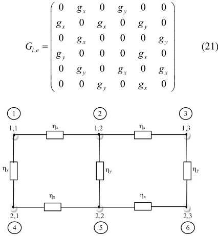
intracellular resistance values along these directions. These resistors arrays were then transformed into matri-ces in the implementation code. This procedure is illus-trated here using 2 by 3 nodes in Figure 3 as an example and the result was generalized to the Nx by Ny nodes

con-sidered in this work.

Each resistor was represented by five indices; the xi and yi indices of one the nodes to which the resistor was

connected, the xj and yj indices of the other nodes to

which the resistor was connected and resistor value η. These two indices were then converted into a single in- dex (encircled numbers in Figure 3) which now repre- sented the first node

 

connected and the second node

 

sistor was connected. It is these two single-indexed num- bers that were stored in the matrices of Gi and Ge to rep-

resent the positions pij where the resistors are to be

placed in the admittance matrices.

Scanning through the network of resistors in Figure 3 from left to right and right to left, it was observed that the resistor values were equal in both directions, that is, η12 is equal to η21 and so on. Based on this, the admi- tance matrices Gi and Ge (6 by 6 matrices) are as shown

in the matrix given by Equation (21).

,

0 0 0

0 0

0 0 0 0

0 0 0 0

0 0 0

0 0 0 0

x y

x x y

0 0

x y

i e

y x

y x x

y x

g g

g g g

g g

G

g g

g g g

g g                      (21)

1,1 1,2 1,3

2,1 2,2 2,3

ηx ηx

ηx ηx

ηy ηy ηy

1 2 3

4 5 6

where gx is 1x and gy is 1y The intracellular and

extracellular admittance matrices Gi and Ge finally

ob-tained represent homogeneous but anisotropic system since the resistors appeared the same everywhere but current flows in the two different directions x and y due to difference in the resistances in the x and y directions were different.

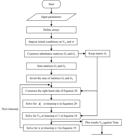
because of its enriched mathematical library and well designed Graphical User Interface (GUI) for displaying graphical representation of results. Another benefit of Java is its portability across various operating systems. The portability however comes with price of slow per- formance in comparison to C/C++. A flow chart for the implementation algorithms is shown in Figure 4 below. Simulation experiments were carried out on a 4GB RAM, Intel (R) Core (TM) i7 CPU M620 @ 2.67GHz and 32-bit operating system computer. Running time of one simulation experiment ranged between 3 and 5 minutes for unchanged and changed parameters.

3.2. Implementation

The discretized equations were implemented in Java programming language (Java 6.0 version). Java is an object-oriented programming language. We adopted Java

Start

Input parameters

Sum matrices Gi and Ge

Invert the sum of matrices Gi and Ge

Construct the right hand side of Equaion 20

Solve for



Solve for Vm at timestep n+1 in Equaion 18

Stop Next timestep

Impose initial conditions on Vm and w

Define arrays

Construct admittance matrices Gi and Ge Keep matrix Gi

Plot results Vm against Time

Solve for w at timestep n+1in Equaion 19

4. SIMULATION RESULTS AND

DISCUSSION

The simulations carried out in this work were grouped into two categories, namely;

 Simulation using the standard values of the basic parameters.

 Simulation using the varying values of the basic parameters.

4.1. Simulation Using the Standard Values of the Basic Parameters

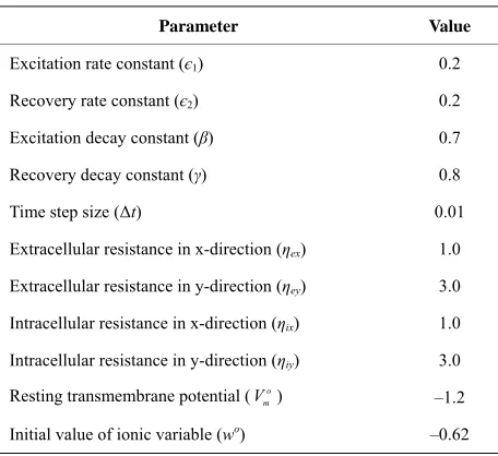
We performed simulation experiment using the devel-oped 2-D Java programme based on the linearized bido-main Equations (18), (19) and (20) and the parameters in Table 1.

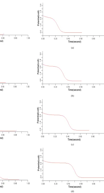
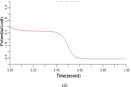
The selected cells 4, 6, 8, 10 of the 50-by-50 nodes (cells) specified in 2-D network domain produced the propagated electrical waves in the normal cardiac tissue as shown in Figures 5(a) to (d) respectively with depo-larization, partial repodepo-larization, plateau, repolarization and resting membrane potential phases identified using the values 0, 1, 2, 3, and 4 in Figure 5(d) for clarity. This electrical signal produced is called the action poten-tial, with the highest period observed in this work around 600 ms. Figures 5(a) to (d) are typically of the same wave pattern, consistent with the theoretical standard and the experimental findings from other researchers [3,24, 25].

4.2. Simulation Using the Varying Values of the Basic Parameters

Here we present the results of simulations we performed to study the effects of the variation of the parameters є1,

Table 1. Values of basic parameters [22].

Parameter Value

Excitation rate constant (є1) 0.2

Recovery rate constant (є2) 0.2

Excitation decay constant (β) 0.7

Recovery decay constant (γ) 0.8

Time step size (Δt) 0.01

Extracellular resistance in x-direction (ηex) 1.0

Extracellular resistance in y-direction (ηey) 3.0

Intracellular resistance in x-direction (ηix) 1.0

Intracellular resistance in y-direction (ηiy) 3.0

Resting transmembrane potential ( o)

m

V –1.2

Initial value of ionic variable (wo_{) –0.62}

(a)

(b)

(c)

0

1

2

3

4

(d)

є2, β and γ that characterizes the adopted FitzHugh-Na- gumo’s ionic model on the electrical wave propagation in the normal cardiac tissue. The standard values consid- ered for these parameters as presented in Table 1 are 0.2, 0.2, 0.7 and 0.8 respectively.

4.2.1. Effects of Variation of є1 and є2 on the

Cardiac Electrical Wave Propagation

The parameters є1 and є2 basically control the dynamics between the transmembrane potential Vm and gating

variable w. In this work, the two parameters had been considered identical. With the value of є1, є2 as 0.2, the electrical wave propagation in the normal cardiac tissue presented in Figure 5 above was obtained. However, when the value of є1, є2 was changed to 0.04 and 0.28 respectively, some differences were observed. At є1, є2 equals 0.04, the electrical wave obtained for cells 4, 6, 8 and 10 have near-infinite slope values when the electrical potential peaks and relaxes. Time dilation effect where the cardiac excitation cycle extends beyond the normal time was also observed. Figures 6(a)-(d) show this ef- fect of decrease value of є1 and є2 on the normal cardiac electrical wave. Comparing Figure 5 and Figure 6, it was observed that each signal in Figure 6 had an ex- tended time for relaxation (resting state) over the corre- sponding signal in Figure 5. The implication of this time dilation effect is that the cardiac tissue has a delayed repolarization, which is an indication of high risk of ar-rhythmia (abnormal cardiac electrical behaviour). If this delay persists, it may result in sudden cardiac death.

With the value of є1, є2 changed to 0.28, no significant differences were observed in terms of excitation time before resting state and shape of signal obtained as com- pared to those of Figure 5. However, it was observed that the signal dwelled more into negative potential be- fore resting. This situation can be regarded as normal since the cell may still be excitable and conduction through the cardiac tissue may not be delayed. Figures 7(a)-(d) show the electrical wave patterns for є1, є2 hav- ing value 0.28.

(a)

(b)

(c)

(d)

Figure 6. Electrical wave propagation in the cardiac tissue for є1=є2=0.04: (a) at cell 4, (b) at cell 6, (c) at cell 8 and (d) at

cell 10.

4.2.2. Effects of Variation of β on the Cardiac Electrical Wave Propagation

(a)

(b)

(c)

(d)

Figure 7. Electrical wave propagation in the cardiac tissue for:

є1, є2 = 0.28 (a) at cell 4, (b) at cell 6, (c) at cell 8 and (d) at cell 10.

(a)

(b)

(c)

(d)

(a)

(b)

(c)

(d)

Figure 9. Electrical wave propagation in the cardiac tissue for

β = 1.1 (a) at cell 4, (b) at cell 6, (c) at cell 8 and (d) at cell 10.

4.2.3. Effects of Variation of γon the Cardiac Electrical Wave Propagation

The effect of variation in the value of γ is similar to that of variation in the value of β. When the value of γ was changed from 0.8 to 0.4 and 1.2 respectively, it was ob- served that variation in the value of γ did not impact any significant effect on the electrical signal as presented in Figures 10 and 11.

Summarily, the results of these simulations showed that of the parameters whose effects of variation on the cardiac electrical wave propagation were studied, it was only decrease in є1, є2 that impacted significantly on the cardiac wave propagation while increase in є1, є2, de- crease or increase in β and γ merely had subtle effect on normal cardiac electrical wave propagation.

(a)

(b)

(d)

Figure 10. Electrical wave propagation in the cardiac tissue for γ= 0.4 (a) at cell 4, (b) at cell 6, (c) at cell 8 and (d) at cell 10.

(a)

(b)

(c)

(d)

Figure 11. Electrical wave propagation in the cardiac tissue for γ= 1.2 (a) at cell 4, (b) at cell 6, (c) at cell 8 and (d) at cell 10.

5. CONCLUSION

In this work, dynamical modelling of cardiac electrical activity using bidomain approach was presented. Apart from the fact that this work has been able to provide some insights into the electrical behaviour of human heart, revealing the nature of the electrical wave propa- gation pattern in the normal cardiac tissue, it also showed that cardiac electrical signal could be significantly af- fected by variation in the values of some of the basic parameters characterizing the adopted FitzHugh-Na- gumo’s ionic model coupling the bidomain model. The simulation results showed the excitation pattern in 2-D. Time dilation effect of the cardiac electrical wave result- ing from decrease in value of є1 and є2 characterizing the ionic model is a sign of potential cardiac arrhythmias and the overall resulting effect is a delayed repolarization, which if persists for a long time may result in sudden cardiac death. The obtained results in this work are very useful in studying the characteristic properties of action potential (the time characteristics of transmembrane po- tential) as it propagates through the cardiac tissue and in effect detect any electrical wave abnormalities in the cardiac tissue. Despite the computational difficulty of numerical simulation of bidomain equations, we were still able to achieve the major objectives of this work by restricting ourselves to 2-D and FitzHugh-Nagumo’s ionic model. In our future work, we will investigate po- tential multiscale and other numerical methods [26,27] for efficient simulation of bidomain equations in 3-D using other ionic models.

REFERENCES

[1] Ekwunife, O.I. and Aguwa, C.N. (2011) A meta-analysis of prevalence rate of hypertension in Nigeria populations.

Journal of Public Health and Epidemiology, 3, 604-607. [2] World Health Organization (2010) Global status report on

http://www.who.int/nmh/publications/ncd_report_full_en. pdf

[3] Wiki (2011) Electrophysiology.

http://en.wikipedia.org/wiki/electrophysiology

[4] DiMasi, J.A., Hansen, R.W. and Grabowski, H.G. (2003) The price of innovation: New estimates of drug develop- ment costs. Journal of Health Economics, 22, 151-185. doi:10.1016/S01676296(02)00126-1

[5] Spiteri, R.J. and Dean, R.C. (2008) On the performance of an implicit-explicit Runge-Kutta method in models of cardiac electrical activity. IEEE Transactions on Bio- medical Engineering, 55, 1488-1495.

doi:10.1109/TBME.2007.914677

[6] Shuaiby, M.S., Mohsen, A.H. and Moumen, E. (2012) Modeling and simulation of the action potential in human cardiac tissue using finite element method. Journal of Communications and Computer Engineering, 2, 21-27. [7] Alin, A.D., Alexandru, M.M., Mihaela, M. and Corina,

M.I. (2011) Numerical simulation in electrocardiography.

Revue Roumaine des Sciences Techniques. Série Électro- technique et Énergétique, 56, 209-218.

[8] Pormann, J.-B., Henriquez, C.S., Board, J.A., Rose, D.J., Harild, D.M. and Henriquez, A.P. (2000) Computer simu- lations of cardiac electrophysiology. ACM/IEEE Super-computing Conference, Duke University, Duke, 4-10 No- vember 2000.

[9] Sundnes, J., Nielsen, B.F., Mardal, K.A., Cai, X., Lines, G.T. and Tveito, A. (2006) On the computational com- plexity of the bidomain and the monodomain models of electrophysiology. Annals of Biomedical Engineering, 34, 1088-1097. doi:10.1007/s10439-006-9082-z

[10] Mark, P., Bruno, D., Jacques, R., Alain, V. and Ramesh, M.G. (2006) A comparison of monodomain and bidomain reaction-diffusion models of action potential in the hu- man heart. IEEE Transactions on Biomedical Engineer- ing, 53, 2425-2435. doi:10.1109/TBME.2006.880875 [11] Bordas, R., Carpentieri, B., Fotia, G., Maggio, F., Nobes,

R., Pitt-Francis, J. and Southern, J. (2009) Simulation of cardiac electrophysiology on next-generation high per- formance computers. Philosophical Transactions of the Royal Society A, 367, 1951-1969.

doi:10.1098/rsta.2008.0298

[12] Linge, S., Southern, J., Hanslien, M., Lines, G.T. and Tveito, A. (2009) Numerical simulation of the bidomain equations. Philosophical Transactions of the Royal Soci- ety A, 367, 1931-1950. doi:10.1098/rsta.2008.0306 [13] Belhamadia, Y. (2010) Recent numerical methods in

electrocardiology. In: Campolo, D., Ed., New Develop-ment in Biomedical Engineering, 151-162.

http://www.intechopen.com/book

[14] Henriquez, C.S. (1993) Simulating the electrical behave- iour of cardiac tissue using the bidomain model. Critical Reviews in Biomedical Engineering, 21, 1-77.

[15] Edminister, J.A. (2006) Electromagnetics. 2nd Edition, Tata McGraw-Hill Publishing Company Limited, New Delhi.

[16] Hayt, W.H. and Buck, J.A. (2006) Engineering electro-magnetics. 7th Edition, McGraw-Hill Education Private Limited, New Delhi.

[17] Reddy, S.R. (2002) Electromagnetic theory. V. Ramesh Publisher, Chennai.

[18] Matthias, G. (2011) 3D bidomain equation for muscle fibers. M.S. Thesis, Fredrich Alexander Universität Er-langen Nürnberg, Germany.

[19] Vigmond, E.J., dosSantos, R.W., Prassl, A.J., Deo, M. and Plank, G. (2008) Solvers for the cardiac bidomain equations. Progress in Biophysics and Molecular Biology, 96, 3-18. doi:10.1016/j.pbiomolbio.2007.07.012

[20] Boulakia, M., Fernandez, M.A., Gerbeau, J.-F. and Zem- zemi, N. (2009) Mathematical modelling of electrocar- diograms: A numerical study. Annals of Biomedical En- gineering, 38, 1071-1097.

doi:10.1007/s10439-009-9873-0

[21] Boulakia, M., Fernandez, M.A., Gerbeau, J.-F. and Zem- zemi, N. (2007) Towards the numerical simulation of electrocardiograms. In: Sachse, F.B. and Seemann, G., Eds., Functional Imaging and Modeling of the Heart, Springer-Verlag, Berlin, 240-249.

[22] Niels, O.F. (2003) Bidomain model of cardiac excitation. http://pages.physics.cornell.edu

[23] Quarteroni, A., Sacco, R. and Saleri, F. (2007) Numerical mathematics. Text in Applied Mathematics, Vol. 37, Springer-Verlag, Berlin.

[24] Nigel, F.H. (1992) Efficient simulation of action potential propagation in a bidomain. Ph.D. Thesis, Duke Univer-sity, Durhan.

[25] Rocha, B.M., Campros, F.O., Planck, G., dos-Santos, R.W., Liebmann, M. and Haase, G.C. (2009) Simulation of electrical activity in the heart with graphical process- ing units. Austria SFB Report No. 2009-016.

[26] Dada, J.O. and Mendes, P. (2011) Multi-scale modelling and simulation in systems biology. Integrative Biology, 3, 86-96. doi:10.1039/c0ib00075b