A Closed Form Approximation for Pricing Temperature Based Weather Derivatives

A Closed-Form Approximation for Pricing

Temperature-Based Weather

Derivatives

A. E. Clements, A. S. Hurn, K. A. Lindsay

School of Economics and Finance, Queensland University of Technology,Brisbane,Australia Email: [email protected], [email protected], [email protected]

Received May 22, 2013; revised June 22, 2013; accepted June 30, 2013

Copyright © 2013 A. E. Clements et al. This is an open access article distributed under the Creative Commons Attribution License, which permits unrestricted use, distribution, and reproduction in any medium, provided the original work is properly cited.

ABSTRACT

This paper develops analytical distributions of temperature indices on which temperature derivatives are written. If the deviations of daily temperatures from their expected values are modelled as an Ornstein-Uhlenbeck process with time- varying variance, then the distributions of the temperature index on which the derivative is written is the sum of trun-cated, correlated Gaussian deviates. The key result of this paper is to provide an analytical approximation to the distri-bution of this sum, thus allowing the accurate computation of payoffs without the need for any simulation. A data set comprising average daily temperature spanning over a hundred years for four Australian cities is used to demonstrate the efficacy of this approach for estimating the payoffs to temperature derivatives. It is demonstrated that expected pay-offs computed directly from historical records are a particularly poor approach to the problem when there are trends in underlying average daily temperature. It is shown that the proposed analytical approach is superior to historical pricing.

Keywords: Weather Derivatives; Temperature Models; Cooling-Degree Days; Distributions for Correlated Variables

1. Introduction

A weather derivative takes its value from an underlying measure of weather, such as temperature, rainfall or snowfall over a particular period of time, and permits the financial risk associated with climatic conditions to be managed. Major participants in this market include utili-ties and insurance companies along with other firms with costs or revenues that are dependent upon the weather. For example, an electricity supplier normally provides its customers with electricity at a fixed price irrespective of the wholesale price. On the other hand the wholesale price of electricity can fluctuate wildly with extreme temperatures, and so temperature-based derivatives can provide a hedging tool for fluctuations in wholesale elec-tricity prices. The first weather derivative was transacted in the US in 1996 and the size of the market now exceeds US$ 8 billion. Almost all weather derivatives are based on temperature indices such as heating degree days and cooling degree days and consequently the focus of this paper will be exclusively on developing closed-form ap-proximations to the distribution of the temperature indi-ces on which temperature-based derivatives are written

which in turn affects their valuation1_.

Traditionally, the valuation of options discounts the expected payoff at the risk-free force of interest based on a zero-arbitrage argument involving the formation of a portfolio consisting of a risk-free combination of an op-tion and the underlying asset [3]. Because temperature cannot be traded, there is no arbitrage-free pricing framework available to price this kind of option. The generally accepted way to value temperature derivatives is the actuarial method in which the fair price is taken to

be the expected value of the payoff ignoring discounting and any volatility premium. The crucial element of this valuation strategy is the accurate calculation of the dis-tribution of the relevant temperature index on which the weather derivative is written.

The most direct way to compute the distribution of temperature indices is from historical records [4,5]. A more elaborate method is to fit a model to the time-series

1_{The first recorded activity was an over-the-counter heating degree day}

of average daily temperature so as to capture seasonal variations in both temperature and its volatility [5,6]. The model is then used to simulate temperature outcomes over the period of the contract in order to construct the distribution of the temperature-based index on which the derivative is written. Note that widely-available mete-orological forecasts are not suitable for this purpose be-cause these forecasts are made over relatively short ho-rizons, such as 7 days, whereas temperature derivatives are often traded well before the contracts generate any payoffs [6-8].

This paper makes two contributions to the existing lit-erature on pricing templit-erature derivatives. First, it builds on the early work of Benth and Šaltynė-Benth [9] by developing closed-form approximations to the distribu-tion of the indices on which temperature-based deriva-tives are written with particular emphasis on obtaining good estimates of the variance of relevant index. Second, two methods are provided for estimating the parameters of the model underpinning the behaviour of temperature that are required to implement the pricing strategy. There are respectively a two-step least-squares based approach and a more comprehensive maximum-likelihood proce-dure.

The ideas developed in this paper are applied to data comprising average daily temperatures for over a century in four Australian cities, namely, Brisbane (BNE), Mel-bourne (MEL), Perth (PER) and Sydney (SYD), where accurate temperature records of long-duration are avail-able at single weather stations. This is a quality data set which represents a substantial improvement on what ap-pears to be the current standard used in the literature. The empirical results based on this data set, demonstrate that the closed-form pricing strategy performs substantially better that using historical pricing.

2. A Model of Daily Temperature

The first step in pricing any temperature-based option must be a model of the underlying index from which the option derives its value, which in the case of temperature derivatives is average daily temperature. Let average daily temperature be expressed as the sum of the seasonal mean temperature T t

( )

at time t and the deviation

of the average daily temperature from its seasonal mean. Suppose that is modelled by the Ornstein- Uhlenbeck process2

( )

t θ

( )

t θ

( )

dθ= −αθdt+σ t d , W α> 0,

,

W s

,

(1.1) where dW is the increment in the Wiener process. The

parameter and the volatility are to be deter-mined from observations of average daily temperature. Equation (1.1) has solution

α σ

( )

t

( )

t _e ( )_{t s}

_{( ) ( )}

_d

t α s

θ − − σ

−∞

=



(1.2) with autocorrelation function at lag u given by

( ) (

)

( )

( )

2 ( ) 2

_{( )}

e ,

e d

u t _{t s}

E t t u S t

S t s s

α

α

θ θ

σ

−

− − −∞

+ =

 

 

=

_

(1.3) where is the variance of daily average tempera-ture. It is straightforward to show that and satisfy

( )

S t

( )

2

t

σ S t

_{( )}

( )

( )

( )

2 d _{2 .}

d

S t

t S

t

σ = + α t

The joint distribution of the average daily temperatures

Tt and t s at the respective calender times t and

is given by the product

T₊

)

(

t+s

)

(

s>0

(

t, t s

)

( )

t,

(

t s, t,

)

f T T₊ = f T t f T₊ t+s T t (1.4)

where f T t

(

t,

)

is the marginal distribution of Tt, namely

( )

(

)

2

1

, exp

2 2π

t t t

t t

T T

f T t

S S

 ₋ 

 

= −

 

 

and

(

)

(

)

(

)

(

)

(

)

2

2

2

1

, ,

2π e

e exp

2 e

t s t

s t s t

s t s t s t t

s t s t

f T t s T t

S S

T T T T

S S

α

α α

+ ₋

+

− + +

− +

+ =

−

 _{− − −} 

 

× _− _

−

 

 

is the transitional probability density function from t

to t . Consequently the joint probability density

func-tion, , in Equation (1.4) becomes

T

s

T₊

(

t, t s

f T T₊

)

(

2

)

e

2π S St t s St

φ

β

−

+ −

where

(

)

(

)(

) (

)

(

)

2 2

2

2 2

t s t t t t t t s t s t t s t s t t s t

S T T S T T T T S T T

S S S

β φ

β

+ + +

+

− − − − + −

=

−

+ + and _β=e−αs

(

T Tt, t s+

. Thus the joint probability density function of

)

is multivariate Gaussian with mean value

(

t, t s+

)

μ= T T and covariance matrix

e . e

s

t t

s

t t s

S S

S S

α α

− −

+

 

Σ = 

 

This model of average daily temperature is now used to develop a closed-form approximation to the distribu-tions of the underlying temperature indices on which

)

T T

)

x

vanilla European options3 _{are written, namely cumulative}

heating degree days (HDDs) and cumulative cooling de-gree days (CDDs).

Let D be the strike of a call option defined as a particular

value of the CDD index. The buyer of this option pays an up-front premium and receives a payout if the value of the CDD index exceeds D at the maturity of the option.

The tick value of a cumulative CDD call option with strike D and duration N days is therefore

3. Distribution of Temperature Indices

Let ave denote the average temperatures in degrees Cel-

sius measured on a particular day at a specific weather station. The HDD and CDD indices at that station on that day are defined respectively by

T

(

max , 0 .

N = CN −D

 (1.7) The per-unit monetary payoff from the contract is its expected tick value

(

)

(

)

ave ave

max ,0 ,

max , 0 ,

HDD T T

CDD T T

= −

= − (1.5) E

[ ]

N _D

(

x D f

) ( )

N x d ,

∞

=

_

−

 (1.8) where f_N

( )

x is the probability density function of CN

and therefore the efficacy of this pricing strategy relies upon the accurate estimation of f_N

( )

x . The idea

pur-sued here is that although the daily contributions to CN

are truncated correlated random variables in which the degree of truncation is nontrivial, nevertheless CN will

behave as a Gaussian random variable provided N is

suitably large. The central theoretical result of the paper is summarized in Proposition 1.

where T˚C is a threshold temperature. The choice of

threshold, in this instance 18˚C, is set by market conven-tion and is the standard used in the US. In the southern (northern) hemisphere the HDD (CDD) season would be from May to September, while the CDD (HDD) season would be from November to March. Without loss of generality, the analysis of this paper will be limited to considering European call options written on cumulative

CDDs. _{Proposition 1}

The CDD index over a period of N consecutive days is

defined by _{cumulative cooling degree days is approximately Gaus-}The tick value CN of a European option defined on

sian distributed with mean value

(

1

, max ,0

N

N k k k

k

C

=

=



  = − (1.6)

[ ]

( ) ( )

1

,

N

N k k k k

k

C S z z φ z

=

 

=



_ Φ + _



where k is the average daily temperature on the

day of the derivative.

T _kth

and variance Var

[ ]

C_N with expression

( )

(

( )

( )

)

(

( )

( )

)

( ) ( )

( )

( )

(

)

[ ] [ ]

(

)

( )

(

)

( )

( )

(

)

₍

₎

(

)

1 1

, ,

1 1

2

, , ,

2 ,

,

2

1 exp

2 1

1 1

N

k k k k k k k k k

N N

j k k j j k j k j k k j k j k

k j j k j k k k k j j k k k j k

k j j k j k k _k

k j k

S z z z z z z z

S S z z z z

z z S S S z S S S z

z z S S S _{p z p z}

q

q q

φ φ

φ χ φ η

β β φ φ η

β

η

= − = = +

_{Φ − + Φ × − − Φ −} 

 

 

+ _ Φ + Φ −



+ + Φ + −

+  ₊  ₊

− Φ − ×Φ_ _

  

+

+ +

 

 



 

   

2 _,

k

z −



  



  

  

 _{ }

 _{ }

where z_k=

(

T_k−T

)

S_k , j k_, e (j k)

α

β ₌ − − _{and the constants}

,

j k

η , _{χj k,} , p and q are defined respectively by

( )

(

)

( )

(

)

, , , , 2 ,

, ₂ , _{2 2}

, ,

, , ,

, , , 1

j j j k k k k j j k j k j k k j k j k j k

j k j k

j k j k

j j k k j j k k j j k k

z S z S z S z S S

p q p

S S S S S S

β β β φ η η

η χ

η φ η

β β β

 

− −

 

= = = − = _ − _

Φ −

− − − _{ }

,

.

η

Φ −

(1.9)

Proposition 1 establishes that accurate closed-form expressions for the mean and the variance of CN are

available in terms of the density function and distribution function of the standard normal distribution alone. Given

these results, the per-unit monetary payoff of a CDD call option is stated in Proposition 2.

Proposition 2

The per-unit monetary payoff of a European call op-tion with strike D written on CN, where the distribution of

CN is Gaussian with mean and variance established in

Proposition 1, is given by

3_{The choice of European option is not limiting in the sense that many}

[ ]

( )

( )

[ ]

[ ]

Var , .

Var

N N

N

C D

C

C

φ ξ ξ ξ+ Φ ξ = −

 

  

The focus of subsequent subsections is to develop and prove the results stated in Proposition 1.

3.1. Mean of CN

It follows directly from Equation (1.6) that

[ ] [ ]

CN = 1 + +

[ ]

N

  

where

(

)

(

)

2

1

[ ] exp d

2 2π

k

k _T

k k

T T

S S

θ θ

∞ _ − 

= − −

 

 





  θ. _(1.10)

Let zk =

(

Tk−T

)

Sk , then the change of variable k k

T S

θ = − z gives immediately

[ ]

(

)

( ) ( )

2₂

e d

2π

, k

z

k z

k k

k k k k

S

z z z

S z z φ z

− −∞

= −

 

= _ Φ + _







(1.11)

where and are respectively the probability density function and cumulative distribution function of the standard normal. The quoted expression for

( )

z

φ Φ

( )

z

[ ]

CN



immediately from result (1.11). Moreover, it

should b

follow

e noted in passing that the proof of Proposition 2 is analogous to the derivation of Equation (1.11).

ppendic

s

3.2. Variance of CN

The computation of the variance of CN is less straight-

forward. The key steps in this calculation are outlined here with the detail being relegated to A es1 and

2. The analysis begins by noting that Var

[ ]

CN can be expressed as the sum of variances in the usual form

j

 (1.12) Straightforward calculation indicates that

and covariances

[ ]

[ ]

1

Var CN N Var k 2N N Cov k, .

−

 

=



 +

 

_ _

1 1 1

k= k= = +j k

[ ]

(

)

(

)

( ) ( )

2 2

2

Var exp d

2 2π

,

k k _T

k k

k k k k 

which u

T T

S S

S z z z

θ

θ _θ

φ

∞ − _ − _

= −

 

 

 

− Φ +





(1.13)

nder the change of variable θ = −T_k S_kz

be-comes

[ ]

(

) ( )

( ) ( )

2

2

Var d

. k

z

k Sk zk z z z

S z z z

φ φ

−∞

= −

k k k k 

− _ Φ + _





(1.14) It is demonstrated in Appendix1 that

 (1.15) thereby completing the computation of the first item on the right hand side of Equation (1.12

The second item on the right hand side of Equation (1.12) is a sum of covariances of generi

( )

(

( )

Var[ ]k =SkΦ zk − φ zk +zkΦ

( )

zk

)

×

(

φ

( )

−zk − Φ −zk

( )

zk

)

). c form

[

]

(

)(

) (

)

[ ] [ ]

Cov t, t s+ _T Tt T Tt s+ T f Tt s+ ,Tt d dT Tt t s+ _{t t s}+ (1.16)

in which t and s (> 0) are to be given appropriate values. First, the integral on the right hand sid

simplified using the change of variables

=

_

− − −

     

e of Equation (1.16) is t t t

T = −T S z and _{t s+ t s+ t s+}

[

]

T =T − S w to get

(

)(

) (

)

[ ] [ ]

Cov  t, t s+ = S St z z zt−z , d dz w− ,

t t s

t s zt s w f zt s zt t t s

+

+ ×

 

−∞ −∞ + − + +

 _{   (1.17)}

where z_t=

(

T_t−T

)

St and zt s+ =

(

Tt s+ −T

)

St s+ and

(

t s, t

)

f z ₊ z probab w,

namely

is the joint ility density of z and

( ), 2

1

e ,

2π

z w

S_{t s −ψ}

t s t

S β S

+ + −

(1.18) where _{β =}e−αs

( )

2

₍

2

₎

2

2

, .

2

t s t t s t s t s t

S z zw S S S w

z w

S S

β ψ

β

+ +

+

− +

=

−

and

+

The integral in Equation (1.17) is expressed as a re-peated integral in which integration is first performed with respect to w and then again with respect to z. The

detailed calculations can be found in Appendix 2, but the outcome of these operations is that

[

]

(

( ) (

)

( ) ( )

)

[ ] [ ]

(

)

( )

(

2

)

( ) ( )

2

Cov

d ,

t t t s t t s t s t s t t t s t

zt t s t s t

t t s t t t s t s t

S S z z z z S S

z S z S

z z S S S z

S S

φ χ φ β

β _{φ β φ φ η}

β

+ + + +

+ +

+ +

−∞

+

Φ + Φ +

 ₋ 

 

× Φ_{ } + −

−

 





(1.19)

where ηt s+ and χt s+ are defined respectively by

2

2

,

.

t s t s t t t s

t s t t t s t s t t s

t s t

z S z S

S S

z S₊ −βz₊ S

(

S S

β η

β

χ

β

+ + +

+ +

+ − =

−

=

−

1.20)

In particular each component of Cov

[

,

]

e eva and cumu andard norma he usefulness t t s+

  , with luated from the the exception of the integral, may b

probability density function lative

dis-tribution function l with

appropriately of

ex-pr

( )

z φ

of the st guments. T

( )

z

Φ chosen ar

ession (1.19) for Cov

[

 t, t s+

]

can be i if the value of the integral appearing in this formula can be expressed, albeit approximate terms of _φ

( )

and

( )

Φ with appropr chosen arguments.

For positive values of the parameter q, this objective

can be achieved by m proximation mproved ly, in

iately aking the ap

(

)

(

( ) ( )22

)

1 e t t ,

t s t

p z z q z z t s

η

+

− − + − +

 

≈ − Φ −

(1.21)

2

t s t s t

z S z S

S S

β β

+ +

 ₋ 

 

Φ_{ }

−

noting, in particular, that the approximation agrees with the interpolated function at and as

dependently of the values of eters

quality of the approximation oved by the values of p and q to ensure first and

de-t

z=z

the param is impr that the

z

= .

z→ −∞ in- p and q. The

choosing second ome of rivatives of the interpolating function match those of the interpolated function when z t The outc this

matching procedure is that

( )

(

)

(

)

( )

2

2

,

t s t

t s t s t

t s

S p

S S

φ η β

η β

η

+ + +

+

= −

Φ − −

 (1.22)

1 t s .

t s

q p η

φ η

+ +



Φ − = _ − _

 

In particular, it is easy to show that The use of the interpolating formula (1.2

the integral in expression (1.19) leads to the conclusion that

0, as required. 1) to evaluate

q>

( ) ( )

( )

(

)

2 2

d

1 _exp 1 _.

zt t s

t t

t t

z z

p z

p z

z z

ξ+ φ

−∞Φ

  

 ₊  ₊

  

≈ Φ − Φ  −



[

]

( ) (

)

( ) ( )

(

)

[ ] [ ]

(

)

( )

(

)

( ) ( )

(

)

(

)

2

2 2

Cov ,

1 1

1 exp

t t s

t t s t t s t s t s t t s t t s t t s t t t t s

t t s t t t s t t s t t s t _t

t t

S S z z z z

z z S S S z

S S S z

z z S S S _{p z}

q q

p z

z

φ χ φ η

β

β φ φ η

β

+

+ + + + +

+ +

+

+ +

+ +

= Φ + Φ

− + + Φ

− −

+  ₊ 

− Φ_ _

+  + 

  ₊ 

  

× −

 

 

 

(1.24)

aced by k and

replaced by j) when substituted into expression

(1.12) provide a closed-form approximation for the vari-ance of the cumulative temperature index which is then treated as a Gaussian random variable with the computed variance and mean value given by expression (1.11).

4. Approximating the Variance

A closed-form expression for the variance of the cumula-tive temperature index was derived in the previous sub-section. Curiously a heuristic argument based on inter-polation can be used to generate a simpler expression for this variance, one that exhibits good accuracy despite the em

by

2 1+q 

 _{ }

 

Expressions (1.15) and (1.24) (with t repl t+s

pirical nature of the derivation. The argument begins noting that the k-th day in the lifetime of a CDD

op-tion will contribute to the cumulative temperature index driving the value of the option with probability

( )

, k ,

k k k k

T T

p z z

S

−

= Φ = (1.25) where Φ

( )

z is the cumulative distribu

the standard normal and T is the tem

tion function of perature above

irst sum-mation on the right hand side of Equation

proximate values

which CDDs are accumulated. If the k-th day always

contributes to the cumulative temperature index then the variance of that contribution would be Sk. On the other

hand if the k-th day never contributes to the cumulative

temperature index then the variance of that contribution would be zero. Since in reality the k-th day contributes

fraction pk of the time then linear interpolation suggests

that the variance of this contribution may be reasonably approximated by Skpk. Based on this idea, the f

(1.12) has

ap-2 1

1 1 q

q+ _ +q_ _ _ + __

(1.23) Expression (1.23) is now incorporated into expression (1.19) to give the final approximate form

[ ]

1 1

Var _{k k k}.

k k

p S

= ≈ =







(1.26) The second summation on the right hand side of Equa-tion (1.12) is a correcEqua-tion to expression (1.26) to take account of the fact that contributions to the value of the temperature index from different days are not

ent. The contribution made by the quantity Cov

[

 t, t s+

]

to the variance of the temperature index is argued in a similar way. In the absence of clipping, the variance of this product is equal to Covθ θk, j with value

( )

e j k k

S −α −

assuming that j>k. However, the product  _{k j} is

nonzero with probability p pk j and therefore the same

linear interpolation argument suggests that Cov k, j

( )

is reasonably approximated by e− j k− _{. Based on} k jSk

α

e righ

p p

mmation on th this idea, the seco

Equation (1.12) has approximate value

nd su t hand side of

( )

1 1

1 1 1 1

2N N Cov , 2N N e j k.

k j k k j k j k k j k

p S p α

− −

− −

formula

= = + = = +

 ≈

 

 

 





(1.27)

In conclusion, linear interpolation suggests that the variance of  is well approximated by the

[ ]

1 ( )

1 1 1

Var N 2N N e j k.

N k k k k j

k k k

C p S p S p α

−

− −

= = = +

=



+





(1.28)

In fact Equatio .28) is the first-order approx ion to the closed-from expressi f the variance in Proposi-tion 1. Consequently, it is expected that this approx tion will perform particularly e level of truncation is low and also when the persistence in tem-perature is low which means that deviatio

j

n (1 imat

on o

ima-well when th

ns in tempera-ture, , are restored to their mean value relativ quic

To test the accuracy of the approximate closed-form ex

( )

t θ

kly.

ely

pression for Var

[ ]

CN stated in Proposition 1, tranches of one millio realizations of Equation (1.1), each of dn u-ration 90 days onstructed for fixed values of and . Specific realization

obt d by d from the m , were c

ally, each rawing _θ0

α

f

σ

aine

(

0

)

, ,

θ θ

arginal density o90 was

θ expressed in the form

( )

_0, 2

N S , and subsequent

values of _θ were determined exactly using the iteration

( )

2 1

e e 2sinh , 1, , ,

k k S k k N

α α

θ − θ − α ξ

−

= + =  (1.29)

where ξk N

( )

0,1 . Realizations of θ

( )

t generated in

this way had mean value zero and stationary standard deviat which was set at 4C˚ for all simulation ex-periments. A t

i

old value of en, say , an

liza

( and a gi

he

generated one million in ndently and identical tributed realizations of C Table 1 shows th

n experime

” and “Std Dev” give the andard de

illion simulations. Estimates of this standard devia-tion based on Proposidevia-tion 1 (Exact) and

ment of Section 1.4 (Approx) are shown.

on S

hresh rea

θ was chos Θ d a cumulative CDD for the 90 day period was con-structed from a tion

(

_θ0, ,_θ90

)

using the for-mula

(

)

90 1

max k , 0 .

k

C θ

=

=



− Θ 1.30) For a given value of α ven value of Θ, each tranc of one million realization of Equation (1.1)

depe DDs.

ly dis-e rdis-esult of seve nts for the case α and thresh-olds Θ∈ −

(

3 , 2 ,S − S −S, 0, , 2 ,3S S S

)

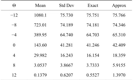
. Table 2 shows the

[image:6.595.307.538.164.302.2]

equivalent result when α=0.5 and the thresholds are unchanged.

Table 1. For α = 0.2 the column headed “Θ” gives threshold temperature relative to zero for contributions to cumulative CDD. Columns headed “Mean

mean cumulative CDD and its st viation based on

one m

0.2

=

the heuristic

argu-Θ Mean Std Dev Exact Approx

−12 1080.1 116.63 116.67 116.69

−8 722.98 114.25 114.23 114.32

−4 99.545 99.272

0 143.57 63.269 61.422

4

389.92 99.608

63.325

29.975 24.680 24.465 23.148

8 3.0560 5.7022 5.3141 6.2514

[image:6.595.308.538.393.531.2]

12 0.1379 0.8556 0.5688 1.4022

Table 2. For α = 0.5 the column headed “Θ” gives threshold temperature relative to zero for contributions to cumulative CDD. Columns headed “Mean” and “Std Dev” give the

mean mulati an dar ation n

one on sim s. E s of anda

ia-tion based on P

gu-ment of Section ppro how

cu ve CDD d its stan d devi based o

milli ulation

roposition 1 (Exact) and the heuristic a

stimate this st rd dev

r

1.4 (A x) are s n.

Θ Mean Std Dev Exact Approx

−12 1080.1 75.730 75.751 75.766

−8 723.01 74.189 74.181 74.346

−4 389.95 64.740 64.703 65.310

0 143.60 41.281 41.246 42.409

4 29.982 16.243 16.154 18.359

8 3.0537 3.8667 3.7333 5.9155

12 0.1379 0.6207 0.5527 1.3970

It is clear from these results that the variance of cumu-lative CDDs predicted by the closed-form approximation

of Pr osition hi pra Min

-ences between the n Proposition 1

and achi y si n b id ly

when e thre emp lies anda ia-tions or more above the mean temperature largely due to the fact that these stances realizations of

CDDs will be val wev is

not a scenario t e pr

The most in ob on i s 1 es

in the cura he c es of

varia . In th of nter is he resh d temp e lies on below t erag ily m

ap

op 1 is ac approxim

eved in ate varia

ctice. ce in

or differ that eved b mulatio ecome ev ent on

th shold t erature two st rd dev under circum

dominated by zero ues. Ho er this hat will b

teresting

occur in servati

actice.

n Table and 2 li unexpected ac cy of t heuristi timate nce

ol

e region eratur

most i or

est, that he av

when t e da th

that, although marginally inferior to the estimates of true variance provided by Proposition 1, are negligibly dif-ferent from it for all practical purposes.

5. Parameter Estimation

To use this model for predicting the payoffs from tem-perature-based derivatives an estimate of the parameter

α in Equation (1.1) is required. This parameter meas-ures the rate at which deviations of temperature from the seasonal are restored to this mean. In order to do so, it is first necessary to obtain estimates of T t

( )

and σ

( )

t .

Following Campbell and Diebold [6], T t

( )

and σ

( )

t

are approximated by the Fourier series

( )

( )

( )

( )

( )

(

0 0 1 2 0

cos sin ,

cos sin

n

k k k k k

n

k k k

T s a b s a s b s

s c c s d

ω ω σ ω = = + + + = + +





)

(1.31)

1 , k k s ω =

where ωk=2kπ 365 and s=0 is assumed to be the

calender date of the first observation of average daily temperature. The contribution b s0 in the expression for

( )

T s is present to take account of any annual trend in

daily average temperature. Otherwise expressions (1.31) assume that seasonal variations in daily average tem-perature follow an annual cycle which is independent of calendar year. Consequently, the expr

corresponding to the expression (1.31) foession for _r 2

( )

S t

( )

s

σ is

( )

0

( )

( )

1

cos sin ,

n

k k k k

k

S s p p ω s q ω s

=

= +



+ (1.32)

where the Fourier coefficients

related to the Fourier coefficien n

by the formulae

Suppose that the data consists of observations average temperatures

0, , , , , ,1 n 1 n

c c  c d 

ts p p0, , ,1 p qn, ,1

d are

,q

0 0

2 ,

2 ,

2 ,

k k k k

k k k

c p q

c p

d p q

α ω

α = _ω + _α 

= _{= − +} 

 (1.33)

where k takes all integer values from k=1 to k=n

inclusive. Two strategies to estimate the value of α and the coefficients in the Fourier series (1.31) are now de-scribed.

5.1. Two-Step Estimator

k

of daily

1, , ,2 N

T T  T at times t t₁, , ,₂ t_N.

The Fourier coefficients of T

(

in a

straightforward way by minimizing t tion

)

s can be estim

he ob

ated jective

func-(

)

(

T t

( )

j

)

.

2

0 0 1 1

1 , , , , , , ,n n N j

j

a b a a b b T

=

Ψ   =



−

the tions n be puted Once these coefficients are known, then devia from the seasonal means ca com

directly from the formula

1, , ,2 n

θ θ θ

( )

j Tj T tj

θ = − . The pr blem is now to find the values of α and the coefficients

0, , ,1

c c 

o which fit the residuals

y bby and Sorensen [12],

1 , , ,

n n

c d  d

, , ,

θ θ θ .

best Bi

1 2 n

Using a result established b

an unbiased estimate ˆα of α is given by the expres-sion

1 1

2 2 2 2

1

n n n n

j

k θ k k

θ θ θ

σ − σ σ− σ

1 1 1 1

2

2

1 1 1 1

. 1

k k j j k j j

n n n

k k j j

θ θ

σ σ σ

= = = − = = = − 1 1 1 2 1 1 2 2 1 1 k k k k k = − − − − − − log    −    − _









    _{  −}   _{ }  







 (1.34) no

Th f

pute the Fourier coefficients

The difficulty, however, in using this expression is that

2

k

σ is unknown whereas what wn is the seasonal variance of the residuals. or finding the values of _α and the coefficients c c₀, , , , , ,₁ c dn ₁ dn

ng. om

is k e strategy is therefore the followi

Step 1: C

and q₁, , qn of S t

( )

directly from the deviations 0 1 n

1, , ,2

, ,

p p p

N

θ θ θ .

Step 2: C compute the from expr rier co

hoose an arbitrary v lue for Fourier coeffi

ession (1.33) with efficients of

a cients

α α=

α

0, ,1

c c

Knowing

, say _α0, and

1 , , ,d

 

the Fo

n n

c d

.

u-0

( )

2 s σ ation (1 pdate the esti

by reco 2 2 en .3 ma m ab 1) te of puting i

les _σ , ,_σ

. Expr n

0

α

n t c c ,cn,

2 2 _to

. This procedure

0, ,1

0 essio urn n be (1.34) is computed f

now used to may then be

d

unt

rom Equ u iterated

1,dn and σ0, ,σn . This procedure is repeated il consecutive estimates of _α are not deemed to be significantly different.

The estimate of _α and the Fourier coefficients a b, , 1, , , , ,n 1 n

a  a b  b and c c₀, ₁, ,c

be

0 0

either

1,

n d dn can

th h

m

the

re from its isfies the

show o the formal used as they stand or can be used as an initial guess for the parameters of e maximum likelihood estimation procedure outlined in t e next subsection.

mean va

tio

5.2. Maximum-Likelihood Estimation

The feasibility of parameter ation by maximum likelihood (ML) in this instance relies on the fact that the transitional probability density function of average daily temperature can be computed under assumption that the deviations of average daily temperatu

lue sat stochastic differential Equation (1.1). Ito’s lemma applied to t stochastic differential Equation (1.1) may be

esti

he n to lead t n

( )

_e ( )j _e ( )

_{( )}

_{d , .}

j

t t t t s

j _t s j

t α α s W t t

θ ₌θ − − ₊ − − σ _>



(1.35)

with θ θj=

( )

tj . The important observation from this

solution is that θ

( )

t is a Gaussian random variable

with mean value

( )

e ( )t tj

j

θ =θ

 

 

( )

_, t_e2 ( )_{t s} 2

_{( )}

_d

t t α s s

χ ₌ − − σ



( )

2 ( )

( )

e ,

j

j

j _t

t t j

S t −α − S t

= −

(1.36)

where the latter expression for χ

( )

t t, j t is derived

di-rectly from the definition of S t

( )

given in Equation

(1.3). Because T=T t

( ) ( )

+θ t , then the average daily

temperature T is itself Gaussian distributed with mean

value

( )

(

)

e ( )t tj

j j

T t + T −T −α − and variance

(

,

)

( )

e2 ( )t tj

( )

j j

t =S t − −α − S t t

χ in which

( )

0 0

( )

( )

1

k=

Thus the average aily temperature T t

( )

has

transi-tional probability

cos sin .

n

k k k k

T t = +a b t+



a ωt +b ω t

d

density function

(1.37)

(

)

e ( )

_{( )}

,

, ,

2π ,

T t j j

j

f T t T t

t t

ψ

χ

−

= , (1.38) where

( )

( )

(

)

( )

(

)

( )

2 e

, .

2 ,

j

t t j j

T T t T

T t

t t

α

ψ

χ

− −

− −

The the sequence

j−T

=

likelihood of observing T T1, , ,2TN

es of average daily temperatures at calendar tim

1, , ,2 N

t t  t is therefore

(

)

(

1 1

)

1

, , .

j j j j j

f T₊ t ₊ T t

= =

∏

0 1 1 0 1 1

1

; , , , , ,_{n n}; , , , , , ,_{n n}

N

a a a b b c c c d d

α

−

   



(1.39)

In practice, the parameters are estimated by minimiz-ing the negative log-likelihood function

( )

(

)

(

)

( )

(

( )

)

1

1

1

1 ₂

1 1

2

1 1 1

2 1

1

1 1

log log 2π log e

2 2

e 1

,

2 _e

j j

j j

j j

N

t t

j j

j

t t N j j j j

t t j

j j

N

S

T T T T

S S

α

α

α

+

+

+

− _{− −}

+ =

− −

− + +

− −

=

+ −

− = + −

− − −

+

−





 S

(1.40) where the notation Sj=S t

( )

j has been used. The

op-timal values for the param of this model are taken to be those which m ession (1.39). Although model (1.1) is s of the intrinsic function

, from a purely oint of view it is e

treat the Fourier coefficients as the parameters

The task is now to provide a means of gauging the effi-cacy of the analytical expressions for the mean and

vari-ance of CN given derived previously in terms of the the

expected payoffs to options contracts. Payoffs based on the analytical results of the paper are compared to h torical pricing as outlined in [4,5]. The metric for co parison is taken to be the mean “profit” of a 90-day call option contract. Profit is defined from the point of view of the buyer of the call option as the difference be

of the contract and the

maximum and minimum

s for cumulative CDDs are

re-ble 3. There are two observations of note

Table 3. First, the distribution of cumulative

eters inimize expr specified in term

technical p of

( )

t σ

to be

asier to

( )

S t

determined by the ML procedure.

6. Empirical Illustration

is-

m-tween the actual tick value expected tick value or “price” of the option. Of course, this is not meant to represent a true price for the option, as this no-tional pricing strategy takes no account of discounting or overhead expenses. But of course, any pricing scheme will stand or fall by its ability to estimate the expected tick value accurately.

6.1. Data

The data set comprises daily

temperature records in degrees Celsius for Brisbane (1/1/ 1887-31/8/2007), Melbourne (1/1/1856-31/8/2007), Perth (1/1/1897-31/8/2007) and Sydney (1/1/1859-31/8/2007). These locations were chosen primarily because they had accurate temperature records of over 100 years duration measured at comparable weather stations4_.

Figure 1 shows the long-term expected values (upper panel) and standard deviations (lower panel) of daily temperatures for each day of the year. The figure shows that the behaviour of the mean and standard deviation is amenable to modelling by a low-order Fourier series ap-proximation. In this exercise the order of the series is taken to be 3. The Fourier approximation is applied only over the period over which the option is to be written, namely, 1 January to 31 March, inclusive.

Descriptive statistic ported in Ta

arising from

CDDs for Melbourne is skewed to the right as evidenced by a mean which is significantly larger than the median. Second, Perth is notable for the diffuse nature of the dis-tribution of cumulative CDDs, recording a standard de-viation significantly larger than those of the other cities.

The distributions of cumulative CDDs for each city is illustrated in Figure 2 which plots both the distribution of historical cumulative CDDs (shaded region) and the predicted distributions for 1950 (dashed line) and 2007 (solid line) generated by closed-form approximations to the distributions of CDDs derived in the paper. To the uniformed eye, the distribution of historical cumulative CDDs may appear well behaved and taken as reasonable evidence in favour of using historical records to price temperature-based derivatives. When compared to the

4_{All the raw data were supplied by Climate Information Services,}

[image:9.595.59.287.84.408.2] [image:9.595.310.538.88.684.2]

Figure 1. The expected value of the average daily tempera-tures (upper panel) and the expected value of the volatility of average daily temperatures (lower panel) are shown for Brisbane, Melbourne, Perth and Sydney.

Table 3. Mean, median, standard deviation, minimum and maximum cumulative CDDs in four Australian cities.

Summary Statistics

N Mean (SD) Med. Min. Max.

BNE 121 584.2 (54.5) 584.6 463.3 705.9

MEL 152 207.9 (64.1) 195.6 93.5 391.4

PER 111 489.6 (83.3) 492.2 298.3 688.3

SYD 149 350.0 (60.1) 350.2 225.5 533.3

distributions for 1950 and 2007 generated by the ana-lytical approach, however, the potential for error inheren

with different strike prices, written on the period 1 January to

t in the historical approach becomes evident. Not only does the mean of the predicted distribution change no-ticeably over time, but the distribution also has lower volatility.

6.2. Payoffs

The profits generated by two call-option contracts

[image:9.595.59.286.494.597.2]

31 March are now reported in Tables 4 and 5 respec-tively. The call options used in the experiment have re-spective strike prices set to be approximately D= +μ

0.5σ and D= +μ 0.75σ where μ

e

[image:10.595.58.286.272.463.2]

tion of CDDs up to the current year under consideration. The experiments begin by pricing these options for the year 1950 using data up to and including 1949. The ac-tual payoff for 1950 is recorded, the profit or loss stored

Table 4. Means and standard deviations of profits to a 90- day call option defined on CDDs with strike price D ap proximately equal to μ + 0.5σ, where μand σ are the un conditional mean and standard deviation of available his-torical CDDs. The option is priced for each year from 1950 to 2007 inclusive.

BNE MEL PER SYD

is the uncondi- devia-tional m an and σ is the unconditional standard

and t upda to include the latest observation on cum ese st re ed up to and incl givi total 8 se e pro or e he means and standard de ations he pro rded easu th orma of each ethods d to ine expected valu

The historical pricing reported in Tables 4 and 5 is

using data for the entire year and the best estimates of th e e us co ng the cl -from appr ations of the stributio of c e CDDs. B ntrast quar vers fo-c the period f 1 Jan ary to t 31 Ma h in

eac its th n a son ianc

v-erage perature for this -day od alon In other words, the fitting procedure is imp nted on the period over which the contract is written. The main reason for adopting this approach is that the behaviour of tem parts e yea elated the pe of the not b allow o infl pa ter estim he mean and variance processes. Another benefit of this approach is tha better resolution of the

mea sses he num of

par

The king c be d from

icing of call options priced on of -m

-Strike D 600 240 530 380

Historical

Mean Payoff −8.1 −14.3 −23.8 7.8

SDev Payoff 33.1 45.8 43.2 48.9

Quarterly Model

Mean Payoff 7.2 13.2 2.2 11.7

SDev Payoff 29.6 41.5 41.8 35.5

Annual Model

Mean Payoff 5.8 15.4 18.3 4.0

SDev Payoff 29.1 41.4 40.0 34.6

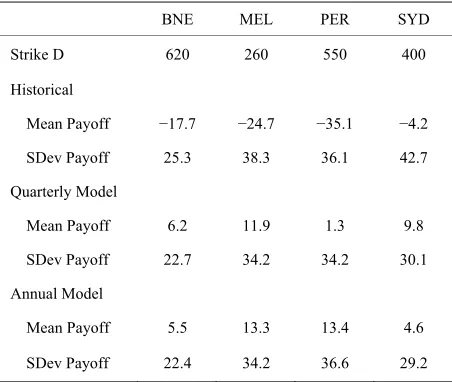
Table 5. Means and standard deviations of profits to a 90- day call option defined on CDDs with strike price D ap-proximately equal to μ + 0.75σ, where μand σare the un-conditional mean and standard deviation of available his-torical CDDs. The option is priced for each year from 1950 to 2007 inclusive.

BNE MEL PER SYD

Strike D 620 260 550 400

Historical

Mean Payoff −17.7 −24.7 −35.1 −4.2

SDev Payoff

Model

off 6. 11.9 1. 9.

Annual

5. 3 13.4 4.

SDev Payoff 22.4 34.2 36.6 29.2 25.3 38.3 36.1 42.7

Quarterly

Mean Pay 2 3 8

SDev Payoff 22.7 34.2 34.2 30.1

Model

Mean Payoff 5 13. 6

the data se ted ulative CDDs uding 2007

. Th ng a

eps are of 5

peat

parat fits f

ach option. T vi of t

fits are rega of the m

as m use

res of determ

e perf nce tick es.

self-explanatory, but the implementation of the closed- form approximations needs further elucidation. Two variations of this method are implemented, namely an annual version and a quarterly version. The annual ap-proach fits the mean and seasonal variance of average daily temperature

e param ters ar ed in mputi osed

umulativ

oxim

y co , the di terly

n ion

usses on rom u he rc

h year and f daily tem

e mea nd sea 90

al var peri

e of a e. leme only

perature in of th r unr to riod option are eing ed t uence rame

ates for t

t

n and variance proce with t same ber ameters.

first stri onclusion to rawn these results is just how bad historical pricing performs for the Australian temperature data. Interestingly enough, it ap-pears that historical pricing in three of the cities has sub-stantially over-priced the call options. This result is counter-intuitive as the conventional view is that there is an upward trend in temperature which would result in the

under-pr the history cu

ulative CDDs.

The resolution of this conundrum is to be found in the behaviour of temperature between the years 1890 and 1920. During this period, Brisbane, Melbourne and Perth recorded substantial outliers in cumulative CDDs, the likes of which were not seen again until late in the sam-ple period. These outliers will have had a disproportion-ate affect on the pricing of temperature derivatives in the 1960s, 1970s and 1980s. Their existence also explains the deterioration of profits based on historical pricing when moving from lower to higher exercise prices. The weather station in Sydney where the temperature data were recorded did not show these extreme temperature events and consequently historical pricing for Sydney performs significantly better.

[image:10.595.59.285.543.734.2]

icing is again a manifestation of the outliers in

ence in performance when moving from th

and with lower standard deviations than historical pricing. Nevertheless, this method appears to underprice some-what, even though these pricing errors are smaller in magnitude than those generated by the historical method. This underpr

cumulative CDDs but in this case, not enough weight is given to them. There is little difference in terms of performance of quarterly and annual models, with the exception of Perth where the quarterly model performs better. It is conjectured that this is due to the ability of the quarterly model to better resolve the extreme tem-perature variations that are prone to take place in Perth. Unlike the case documented for historical pricing, there seems little differ

e lower to the higher exercise price for the the closed- form approach.

7. Conclusions

This paper has derived closed-form expressions for ap-proximating the distribution of temperature indices. The major practical use for these approximations is in esti-mating the payoffs to temperature-based weather deriva-tives. Although the cumulative cooling degree day index is the focus of this research, the methods used are equally applicable to derivatives based on cumulative heating degree days. Common practice when modelling average daily temperature is to regard the deviations of tempera-ture from its expected value as an Ornstein-Uhlenbeck process. The key result derived in this paper, is that if this model of temperature is adopted, then the distribu-tion of cumulative cooling degree days may be con-structed as the sum of truncated, correlated Gaussian deviates. The mean and variance of the resultant Gaus-sian distribution depend on the parameters of the under-lying temperature process and its autocorrelation struc-ture.

The efficacy of these approximate distributions is tested by estimating the payoffs to temperature-based derivatives. Time series data spanning over a hundred years of average daily temperatures in four major Austra-lian cities are used to estimate the payoffs to European call options written on cooling degree days. The robust conclusion to emerge from this line of research is that the closed-form distributions perform more reliably than the

historical pricing method that is commonly advocated in the literature.

REFERENCES

[1] J. Tindall, “Weather Derivatives: Pricing and Risk Man- agement Applications,” Institute of Actuaries of Australia, Unpublished Manuscript, 2006.

[2] M. Garman, C. Blanco and R. Erickson, “Weather De-rivatives: Instruments and Pricing Issues,” Environmental Finance, 2000.

[3] F. Black and M. Scholes, “The Pricing of Options and Corporate Liabilities,” Journal of Political Economy, Vol. 81, 1973, pp. 637-659. doi:10.1086/260062

[4] L. Zeng, “Pricing Weather Derivatives,” Journal of Risk Finance, Vol. 81, No. 3, 2000, pp. 72-78.

doi:10.1108/eb043449

[5] E. Platen and J. West, “Fair Pricing of Weather Deriva-tives,” Quantitative Finance Research Centre, University of Technology Sydney, Research Paper Series, 106, 2003. [6] S. D. Campbell and F. X. Diebold, “Weather Forecasting for Weather Derivatives,” Journal of the American Statis- tical Society, Vol. 100, 2005, pp. 6-16.

[7] D. S. Wilks, “Statistical Methods in the Atmospheric Sciences,” Academic Press, New York, 1995.

[8] S. Jewson and of Weather Fore-

casts in the Pri tives,” Meterologi- R. Caballero, “The Use

cing of Weather Deriva

cal Applications, Vol. 10, No. 4, 2003, pp. 377-389.

doi:10.1017/S1350482703001099

[9] F. E. Benth and J. Šaltynė-Benth, “Stochastic Modelling of Temperature Variations with a View Toward Weather Derivatives,” Applied Mathematical Finance, Vol. 12, No. 1, 2005, pp. 53-85.

doi:10.1080/1350486042000271638

[10] M. H. A. Davis, “Pricing Weather Derivatives by Mar- ginal Value,” Quantitative Finance, Vol. 1, 2001, pp. 1-4.

doi:10.1080/713665730

[11] P. Alaton, B. Djehiche and D. Stillberger, “

and Pricing Weather Derivatives,” Applied Mathematical On Modelling Finance, Vol. 9, No. 1, 2002, pp. 1-20.

doi:10.1080/13504860210132897

[12] B. M. Bibby and M. Sorensen, “Martingale Estimation Functions for Discretely Observed Diffusion Processes,” Bernoulli, Vol. 1, No. 1/2, 1995, pp. 17-39.