A plug in averaging estimator for regressions with heteroskedastic errors

Munich Personal RePEc Archive

A plug-in averaging estimator for

regressions with heteroskedastic errors

LIU, CHU-AN

National University of Singapore

10 August 2012

A Plug-In Averaging Estimator for Regressions

with Heteroskedastic Errors

Chu-An Liu∗

National University of Singapore†

[email protected] August 10, 2012

Abstract

This paper proposes a new model averaging estimator for the linear regression model with het-eroskedastic errors. We address the issues of how to optimally assign the weights for candidate models and how to make inference based on the averaging estimator. We derive the asymptotic mean squared error (AMSE) of the averaging estimator in a local asymptotic framework, and then choose the optimal weights by minimizing the AMSE. We propose a plug-in estimator of the optimal weights and use these estimated weights to construct a plug-in averaging estimator of the parameter of interest. We derive the asymptotic distribution of the plug-in averaging estimator and suggest a plug-in method to construct confidence intervals. Monte Carlo simulations show that the plug-in averaging estimator has much smaller expected squared error, maximum risk, and maximum regret than other existing model selection and model averaging methods. As an empirical illustration, the proposed methodology is applied to cross-country growth regressions.

Keywords: Local asymptotic theory, Model averaging, Model selection, Plug-in estimators. JEL Classification: C51, C52.

∗_{I am deeply indebted to Bruce Hansen and Jack Porter for guidance and encouragement. I also thank Xiaoxia}

Shi, Biing-Shen Kuo, Yu-Chin Hsu for helpful discussions.

1

Introduction

In recent years, interest has increased in model averaging from the frequentist perspective. Unlike model selection, which picks a single model among the candidate models, model averaging incor-porates all available information by averaging over all potential models. Model averaging is more robust than model selection since the averaging estimator considers the uncertainty across different models as well as the model bias from each candidate model. The central questions of concern are how to optimally assign the weights for candidate models and how to make inference based on the averaging estimator. This paper proposes a plug-in averaging estimator to resolve both of these issues. We derive the asymptotic mean squared error (AMSE) of the averaging estimator in a local asymptotic framework. We show that the optimal model weights which minimize the AMSE depend on the local parameters and the covariance matrix. The idea of the plug-in averaging esti-mator is to estimate the infeasible optimal weights by minimizing the sample analog of the AMSE. We show that the plug-in averaging estimator has a non-standard asymptotic distribution. Hence, confidence intervals based on normal approximations lead to distorted inference in this context. We suggest a plug-in method to construct confidence intervals, which have good finite-sample coverage probabilities.

Empirical studies often must consider whether additional regressors should be included in the baseline model. Adding more regressors reduces the model bias but causes a large variance. To address the trade-off between bias and variance, this paper studies model averaging in a local asymptotic framework where the regression coefficients are in a local n−1/2 _{neighborhood of zero.}

Under drifting sequences of parameters, the AMSE of the averaging estimator remains finite and provides a good approximation to the finite sample MSE. The O(n−1/2) framework is canonical in the sense that both squared model biases and estimator variances have the same order O(n−1_).

Therefore, the optimal model is the one that has the best trade-off between squared model biases and estimator variances. The local-to-zero framework is crucial to analyze the asymptotic distribution of the averaging estimator. If all regression coefficients are fixed, then the model bias term tends to infinity and dominates the limiting distribution. In such a situation, the model which includes all regressors is the only one we should consider. The local asymptotic framework also implies that all of the candidate models are close to each other as the sample size increases. Hence, it is informative to employ model averaging rather than model selection in this framework.

normal random vector.

In addition to the plug-in averaging estimator, we also derive the asymptotic distributions of the Akaike information criterion (AIC) selection estimator (Akaike, 1973), the smoothed AIC (S-AIC) model averaging estimator (Buckland, Burnham, and Augustin, 1997), and the Jackknife Model Averaging (JMA) estimator (Hansen and Racine, 2012) in the local asymptotic framework. Although the asymptotic distribution of the averaging estimator with data-driven weights is non-standard, it can be approximated by simulation. Numerical comparisons show that the plug-in averaging estimator has substantially smaller risk than other data-driven averaging estimators in most ranges of the parameter space.

The empirical literature tends to focus on one particular parameter instead of assessing the overall properties of the model. In contrast to most existing model selection and model averaging methods, our method is tailored to the parameter of interest. The proposed averaging estimator is constructed based on the focus parameter instead of the global fit of the model. The focus parameter is a smooth real-valued function of regression coefficients. Thus, we focus attention on a low-dimension function of the model parameters. Also, we allow different model weights to be chosen for different parameters of interest.

One straightforward way to construct the confidence interval for the focus parameter is to employ the t-statistic. The confidence interval is constructed by inverting the t-statistic based on the parameter of interest. We show that the asymptotic distribution of the model averaging t-statistic depends on unknown local parameters, and thus cannot be directly used for inference. We propose a plug-in method to construct the confidence interval based on a non-standard limiting distribution. The idea is to simulate the limiting distribution of the model averaging t-statistic by replacing the unknown parameters with plug-in estimators. The confidence interval is constructed based on the 1₋αquantile of the simulated distribution. Our simulations show that the coverage probability of the plug-in confidence interval is close to the nominal level, while the confidence interval based on normal approximations leads to distorted inference.

The idea of using the local asymptotic framework to investigate the limiting distributions of model averaging estimators is developed by Hjort and Claeskens (2003) and Claeskens and Hjort (2008). However, their work is limited to the likelihood-based model. Following Hjort and Claeskens (2003), DiTraglia (2011) proposes a moment selection criterion and a moment averaging estimator for the GMM framework. Like DiTraglia, we employ a drifting asymptotic framework to approxi-mate the finite sample MSE. Unlike DiTraglia, we consider model averaging rather than moment averaging, and we combine the models with valid moment conditions rather than potentially in-valid moment conditions. Other work on the asymptotic properties of averaging estimators includes Leung and Barron (2006), P¨otscher (2006), and Hansen (2009, 2010). Leung and Barron (2006) study the risk bound of the averaging estimator under a normal error assumption. P¨otscher (2006) analyzes the finite sample and asymptotic distributions of the averaging estimator for the two-model case. Hansen (2009) evaluates the AMSE of averaging estimators for the linear regression model with a possible structural break. Hansen (2010) examines the AMSE and forecast expected squared error of averaging estimators in an autoregressive model with a near unit root in a local-to-unity framework. Most of these studies, however, are limited to the two-model case and the homoskedastic framework.

There is a large literature on inference after model selection, including P¨otscher (1991), Kabaila (1995, 1998), Leeb and P¨otscher (2003, 2005, 2006, 2008). These papers point out that the coverage probability of the confidence interval based on the model selection estimator is lower than the nominal level. They also argue that the conditional and unconditional distribution of post-model-selection estimators cannot be uniformly consistently estimated. In the model averaging literature, Hjort and Claeskens (2003) and Claeskens and Hjort (2008) show that the traditional confidence interval based on normal approximations leads to distorted inference. P¨otscher (2006) argues that the finite-sample distribution of the averaging estimator cannot be uniformly consistently estimated. There are also alternatives to model selection and model averaging. Tibshirani (1996) introduces the LASSO estimator, a method for simultaneous estimation and variable selection. Zou (2006) proposes the adaptive LASSO approach and presents its oracle properties. White and Lu (2010) propose a new Hausman (1978) type test of robustness for the core regression coefficients. They also provide a feasible optimally combined GLS estimator. Hansen, Lunde, and Nason (2011) propose the model confidence set which is constructed based on an equivalence test.

2

Model and Estimation

Consider a linear regression model

yi=x′iβ+z′iγ+ei, (2.1)

E(e_i|xi,zi) = 0, (2.2)

E(e2_i|xi,zi) =σ2(xi,zi), (2.3)

where yi is a scalar dependent variable, xi = (x1i, ..., xki)′ and zi = (z1i, ..., zℓi)′ are vectors of

regressors,ei is an unobservable regression error, andβ(k×1) andγ(ℓ×1) are unknown parameter

vectors. The error term is allowed to be heteroskedastic and there is no further assumption on the distribution of the error term. Here, xi are the core regressors which must be included in the

model based on theoretical grounds, whilezi are the auxiliary regressors which may or may not be

included in the model. Note that xi may only include a constant term or even an empty matrix.

In matrix notation, we write the model as

y=Xβ+Zγ+e=Hθ+e (2.4)

whereH= (X,Z) and θ= (β′,γ′)′.

The parameter of interest isµ=µ(θ) =µ(β,γ), which is a smooth real-valued function. Unlike the traditional model selection and model averaging approaches which assess the global fit of the model, we evaluate the model based on the focus parameterµ. For example,µmay be an individual coefficient or a ratio of two coefficients of regressors.

Let M be the number of submodels, where the submodel includes all core regressors X and a subset of auxiliary regressors Z. The m’th submodel has k+ℓm regressors. If we consider a

sequence of nested models, then M = ℓ+ 1. If we consider all possible submodels, then M = 2ℓ_.

LetΠm be the ℓm×ℓselection matrix which selects the included auxiliary regressors. Here, ℓm is

the number of auxiliary regressors zi included in the submodelm.

The least-squares estimator of θ for the full model, i.e. all auxiliary regressors are included in the model, is

ˆ

θ= βˆ

ˆ

γ

!

= (H′H)−1H′y, (2.5)

and the estimator for the submodelm is

˜

θm=

˜

βm

˜

γ_m

!

= (H′_mHm)−1H′my, (2.6)

where Hm = (X,ZΠ′m) with m = 1, ..., M. Let I denote an identity matrix and0 a zero matrix.

If Πm =Iℓ, then we have θ˜m = (H′H)−1H′y =θˆ, the least-squares estimator for the full model.

IfΠm =0, then we haveθ˜m = (X′X)−1X′y, the least-squares estimator for the narrow model, or

We now define the averaging estimator of the focus parameter µ. Let w= (w1, ..., wM)′ be a

weight vector with wm ≥0 and PMm=1wm = 1. That is, the weight vector lies in the unit simplex

inRM:

Hn=

(

w_∈[0,1]M :

M

X

m=1

wm= 1

)

.

The sum of the weight vector is required to be one. Otherwise, the averaging estimator is not consistent. Let ˜µm=µ(θ˜m) =µ(β˜m,γ˜m) denote the submodel estimates. The averaging estimator

of µis

¯ µ(w) =

M

X

m=1

wmµ˜m. (2.7)

Here we want to point out that we have less restrictions on the weight function than other existing methods. Leung and Barron (2006), P¨otscher (2006), and Liang, Zou, Wan, and Zhang (2011) assume the parametric form of the weight function. Hansen (2007) and Hansen and Racine (2012) restrict the weights to be discrete. Contrary to these works, we allow continuous weights without assuming any parametric form, which is more general and applicable than other approaches.

3

Asymptotic Properties

To establish the asymptotic distribution of the averaging estimator, we follow Hjort and Claeskens (2003) and use a local-to-zero asymptotic framework where the auxiliary parametersγare in a local n−1/2 _{neighborhood of zero. Leth}

i = (x′i,z′i)′ andQ= E (hih′i) partitioned so that E (xix′i) =Qxx, E (xiz′i) =Qxz, and E (ziz′_i) = Qzz. Let Ω= limn→∞n−1

Pn i=1

Pn

j=1E hih′jeiej partitioned so

that limn→∞n−1Pni=1

Pn

j=1E xix′jeiej =Ωxx, limn→∞n

−1Pn i=1

Pn

j=1E xiz′jeiej=Ωxz, and limn→∞n−1Pn_i=1Pn_j=1E ziz′jeiej=Ωzz. Note that if the error term ei is serially uncorrelated, Ωcan be simplified asΩ= E hih′ie2i

.

Assumption 1. Asn_{→ ∞},n1/2γ=n1/2γn→δ∈Rℓ.

Assumption 2. Asn_{→ ∞},n−1_H′_H−→p _{Q and n}−1/2_H′_e−→d _{R∼N(0,Ω).}

Assumption 1 is the key assumption to develop the asymptotic distribution. It is a common assumption in the weak instrument literature, see Staiger and Stock (1997). This assumption says the partial correlations between the auxiliary regressors and the dependent variable are weak. This assumption implies that as the sample size increases, all of the submodels are close to each other. Under this framework, it is informative to know if we can do better by averaging the candidate models, instead of choosing one single model. Also note that theO(n−1/2_{) framework gives squared}

Assumption 2 is a high-level condition which permits the application of cross-section, panel, and time-series data. This condition holds under appropriate primitive assumptions. For example, ifyi is a stationary and ergodic martingale difference sequence with finite fourth moments, then the

condition follows from the weak law of large numbers and the central limit theorem for martingale difference sequences.

Since the selection matrix Πm is non-random with elements either 0 or 1, for the submodel m

we have n−1H′_mHm p

−→Qm whereQm is nonsingular with

Qm =

Qxx QxzΠ′_m ΠmQzx ΠmQzzΠ

′ m

!

,

and n−1/2_H′ me

d

−→N(0,Ωm) with

Ωm =

Ωxx ΩxzΠ

′ m

ΠmΩzx ΠmΩzzΠ′_m

!

.

Let θm = (β′,γm′ )′ = (β′,γ′Π′m)′. In this section, we concentrate on fixed weights. The

averaging estimator with data-driven weights is presented in the next section. The following lemmas describe the asymptotic distributions of the least-squares estimators and the limiting distribution of the focus parameter.

Lemma 1. Suppose Assumptions 1-2 hold. As n_{→ ∞}, we have

√

nθˆ₋θ_−→d Q−1R_∼N 0,Q−1ΩQ−1,

√

nθ˜_m−θ_m−→d Amδ+BmR∼N Amδ, Q−m1ΩmQ−m1

,

where

Am =Q−m1

Qxz ΠmQzz

!

Iℓ−Π′mΠm, Bm =Q−m1S′m, and Sm =

Ik 0k×ℓm 0ℓ×k Π′m

!

.

Note that Sm is an extended selection matrix of dimension (k+ℓ)×(k+ℓm). Denote Dθm =

D′_β,D′_γm′, Dβ = ∂µ/∂β, and Dγm = ∂µ/∂γm with partial derivatives evaluated at the null points (β′,0′)′.

Lemma 2. Suppose Assumptions 1-2 hold. As n_{→ ∞}, we have

√

nµ(θ˜m)−µ(θ)

_d

−→Λm =a′mδ+b′mR∼N a′mδ, D′θmQ

−1

m ΩmQ−m1Dθm

,

where

am = Iℓ−Π′mΠm

Qzx

QzzΠ′_m

!

Q−_m1Dθm−Dγ

!

The main difference between Lemma 1 and 2 is the asymptotic distribution of the focus pa-rameter involves the partial derivatives. Note that both Amδand a′mδrepresent the bias terms of

submodel estimators. To be more precise, the biases come from the omitted auxiliary regressors. As we can see from (Iℓ−Π′mΠm), this is the selection matrix which selects the omitted auxiliary

regressors.

Lemma 1 and 2 imply joint convergence in distribution of all submodels since all asymptotic distributions of submodels can be expressed in terms of the same normal random vector R. The following theorem shows the asymptotic normality of the averaging estimator with fixed weights.

Theorem 1. Suppose Assumptions 1-2 hold. As n_{→ ∞}, we have

√

n(¯µ(w)₋µ)_−→d N a′δ, V where

a=

M

X

m=1

wmam,

V =

M

X

m=1

w_m2D′_θmQ_m−1ΩmQ−m1Dθm+ 2

X

m<p

wmwpD′θmQ

−1

m Ωm,pQ−p1Dθp,

Ωm,p=

Ωxx ΩxzΠ

′ p

ΠmΩzx ΠmΩzzΠ′_p

!

,

and am is defined in Lemma 2.

Following by Theorem 1, we can derive the AMSE of the averaging estimator. Here, we define the AMSE as AMSE(ˆµ) = limn→∞E n(ˆµ−µ)2. Then the AMSE of the averaging estimator (2.7)

is

AMSE(¯µ(w)) =w′ζw (3.1)

whereζ is anM _×M matrix with the (m, p)th element

ζm,p =δ′ama′pδ+D′θmQ

−1

m Ωm,pQ−p1Dθp (3.2)

wheream is defined in Lemma 2 and Ωm,p is defined in Theorem 1.

The optimal fixed-weight vector is the value which minimizes AMSE(¯µ(w)) over w_{∈ Hn}:

wo= argmin w∈H_n

w′ζw. (3.3)

4

Plug-In Averaging Estimator

The optimal fixed weights derived in the previous section are infeasible, since they depend on the unknown parameters,Dθm,Qm, Ωm,p,am, and δ. Furthermore, the optimal fixed weights cannot be estimated directly because there is no closed form expression when the number of models is greater than two. A straightforward solution is to estimate the AMSE of the averaging estimator given in (3.1) and (3.2), and to choose the data-driven weights by minimizing the sample analog of the AMSE.

The plug-in estimator of AMSE(¯µ(w)) is w′ζˆw where ζˆ is the sample analog of ζ with the (m, p)th element

ˆ

ζm,p=δˆ′ˆamˆa′pδˆ+Dˆ′θmQˆ

−1

m Ωˆm,pQˆ−p1Dˆθp.

The weight vector of the plug-in estimator is defined as

ˆ

wpia= argmin

w∈H_n

w′ζˆw. (4.1)

The plug-in averaging estimator is

¯

µ(wˆpia) = M

X

m=1

ˆ

wpia,mµ˜m. (4.2)

We now discuss the plug-in estimator ˆζm,p. We first consider the estimator of Dθm. Let ˆ

Dθm = S

′

mDˆθ and Dˆθ = ∂µ(θˆ)/∂θ where Sm defined in Lemma 1 is a non-random selection

matrix and θˆ is the estimate from the full model. By Lemma 1 and the continuous mapping theorem, it follows that Dˆθm is a consistent estimator of Dθm.

Next, we consider the estimators of Qm,Ωm,p, and am. Let Qˆm =Sm′ QSˆ m, Ωˆm,p =S′mΩSˆ p,

and

ˆ

am = Iℓ−Π′mΠm

ˆ Qzx ˆ QzzΠ′_m

!

ˆ

Q−_m1Dˆθm−Dˆγ

!

. (4.3)

Consistent estimators for Qm, Ωm,p, and am are available, since these unknown parameters are

functions of the covariance matrix Q and Ω. We use the method of moments estimators for Q and Ω. Let Qˆ = n−1P_in₌₁hih′i and it follows that Qˆ

p

−→ Q. If the error term ei is serially

uncorrelated, thenΩcan be estimated consistently by the heteroskedasticity-consistent covariance matrix estimator

ˆ Ω= 1

n

n

X

i=1

hih′ieˆ2i, (4.4)

which is proposed by White (1980). Here ˆei =yi−xi′βˆ−z′iγˆ is the least squares residual from the

heteroskedasticity and autocorrelation consistent covariance matrix estimator

ˆ Ω=

n

X

j=−n

k(j/Sn)ˆΓ(j), (4.5)

ˆ

Γ(j) = 1 n

n−j

X

i=1

hih′i+jˆeieˆi+j, forj≥0, (4.6)

ˆ

Γ(j) =Γ(ˆ ₋j)′, forj <0, (4.7)

wherek(_·) is a kernel function andSn the bandwidth. Under some regularity conditions, it follows

thatΩˆ _−→p Ω; for serially uncorrelated errors, see White (1980) and White (1984), and for serially correlated errors, see Newey and West (1987) and Andrews (1991b). By the continuous mapping theorem and the fact that the selection matrix is non-random, it follows thatQˆm

p

−→Qm,Ωˆm,p p −→

Ωm,p, and ˆam p −→am.

We now consider the estimator for the local parameter δ. Unlike Dθm, Qm, Ωm,p, and am, there is no consistent estimator for the parameter δ. This implies that the optimal weights cannot be estimated consistently. We propose to use the asymptotically unbiased estimator for δ. Let ˆ

δ=√nγˆ whereγˆ are the estimates from the full model. From Lemma 1, we have

ˆ

δ=√nγˆ _−→d Rδ=δ+ΠℓQ−1R∼N(δ,ΠℓQ−1ΩQ−1Π′ℓ) (4.8)

where Π_ℓ = (0ℓ×k,Iℓ). As shown above, δˆ is an asymptotically unbiased estimator for δ. The

limiting distribution of the plug-in estimatorδˆisRδwhich is a linear function of the normal random

vector R. We use this result to establish the asymptotic distribution of the plug-in averaging estimator.

Note that the first term of ζm,p can be rewritten as a′mδδ′ap. Hence, we can estimate δδ′

instead of δ. Since RδR′δ has mean δδ′+ΠℓQ−1ΩQ−1Π′ℓ, another possible estimator is nˆγγˆ′−

ΠℓQˆ−1Ω ˆˆQ−1Π′ℓ forδδ′. However, it might happen that the estimator of the squared bias terms,

the diagonal terms of δδ′, are negative. Furthermore, the asymptotic distribution of the squared bias estimator is more complicated. Therefore, we only consider the estimator δˆ.

The following assumption is imposed on the estimator of the covariance matrix.

Assumption 3. There existsΩˆ such thatΩˆ _−→p Ω.

Assumption 3 is a high-level condition on the estimator of the covariance matrix. Rather than impose regularity conditions, we assume there exists a consistent estimator for Ω. The consistent estimators for the covariance matrix are given in (4.4) and (4.5) for serially uncorrelated errors and serially correlated errors, respectively. The sufficient condition for the consistency is ei is i.i.d. or

a martingale difference sequence with finite fourth moment. For serial correlation, data is a mean zero α-mixing or ϕ-mixing sequence.

Theorem 2. Suppose Assumptions 1-3 hold. As n_{→ ∞}, we have

where ζ∗ is anM _×M matrix with the (m, p)th element

ζ_m,p∗ =R′_δama′pRδ+D′θmQ

−1

m Ωm,pQ−p1Dθp

and Rδ=δ+ΠℓQ−1R. Also, we have

ˆ

wpia−→d wpia∗ = argmin

w∈H_n

w′ζ∗w, (4.9)

and

√

n µ¯(wˆpia)−µ−→d M

X

m=1

w∗_pia,mΛm (4.10)

where Λm=a′mδ+b′mR.

Theorem 2 shows that the estimated weights are asymptotically random. In order to derive the asymptotic distribution of the plug-in averaging estimator, we show that there is joint convergence in distribution of all submodel estimators ˜µm and estimated weightswˆpia. The joint convergence in

distribution comes from the fact that both Λm and wpia,m∗ can be expressed in terms of the normal

random vector R. It turns out the limiting distribution of the plug-in averaging estimator is not normally distributed. Instead, it is a non-linear function of the normal random vectorR.

The non-normal nature of the limiting distribution of the averaging estimator with data-driven weights is also pointed out by Hjort and Claeskens (2003) and Claeskens and Hjort (2008). The result is useful to construct the confidence interval.

5

AIC, S-AIC and JMA Estimators

In this section, we present the asymptotic distributions of the AIC model selection estimator, the S-AIC model averaging estimator, and the Jackknife Model Averaging estimator. The limiting dis-tributions of AIC, S-AIC, and JMA estimators are non-standard in the local asymptotic framework. We also present the results of the two-model case.

5.1 AIC and Smoothed AIC

The model selection estimator based on information criteria is a special case of the model averaging estimator. The model selection puts the whole weight on the model with the smallest value of the information criterion and give other models zero weight. Hence, the weight function of the model selection estimator can be described by the indicator function.

The AIC for the linear regression model (2.4) is

where ˜σ2_m =n−1Pn_i=1e˜2_mi and ˜emi are the least squares residuals from the submodel m, that is,

˜

emi=yi−x′iβ˜m−z′miγ˜m and zmi =Πmzi. The AIC model selection estimator is thus

¯

µ(wˆaic) = M

X

m=1

ˆ

waic,mµ˜m,

ˆ

waic,m=1{AICm = min(AIC1,AIC2, ...,AICM)}.

Instead of estimating the regression function based on a single model, the S-AIC model av-eraging estimator proposed by Buckland, Burnham, and Augustin (1997) assigns the weights of each candidate models by using the exponential Akaike information criterion. The weight for each submodel is proportional to the log-likelihood of model. The S-AIC model averaging estimator is defined as

¯

µ(wˆsaic) = M

X

m=1

ˆ

wsaic,mµ˜m, (5.1)

ˆ

wsaic,m =

exp(₋1₂AICm)

PM

m=1exp(−12AICm)

. (5.2)

The S-AIC weight is similar to the smoothed Bayesian information criterion (S-BIC) model av-eraging where the weights are chosen by using the exponential Bayesian information criterion. The S-BIC weight is exp(₋1₂BICm)/PM_m=1exp(−1₂BICm), where BICm =nlog(˜σ2m) + log(n)(k+ℓm).

The weights of the Bayesian model averaging are interpreted as the posterior model probabilities. Therefore, the S-AIC weight may be interpreted as the model probability.

The S-AIC model averaging estimator is appealing because of its simplicity. Also, there is a closed form expression of the S-AIC weights for any number of submodels. However, both AIC and S-AIC are not robust for heteroskedastic regressions. The misspecification-robust version of AIC is Takeuchi information criterion, see Burnham and Anderson (2002). Furthermore, the S-AIC weights ignore the covariances between the submodel estimators. Also, the S-S-AIC weights are formed based on the global fit of the model, and the weights does not adjust according to the parameter of interest.

Hjort and Claeskens (2003) and Claeskens and Hjort (2008) show the limiting distributions of the AIC model selection estimator and the S-AIC model averaging estimator in the likelihood framework. Let AIC_∅ be the AIC for the narrow model. Following Theorem 5.4 of Claeskens and Hjort (2008), we can show that the

AIC_∅−AICm−→d R′δΣmRδ−2(k+ℓm) (5.3)

whereΣm=V_δ−1Πm′ ΠmV_δ−1Π′m

−1

ΠmV_δ−1 and Vδ=ΠℓQ−1ΩQ−1Π′ℓ.

Note that (5.3) can be expressed as G′ΨmG−2(k+ℓm) whereG∼N(Vδ−1/2δ,Iℓ) andΨm=

V_δ−1/2Π′_m ΠmVδ−1Π′m

−1

ΠmVδ−1/2. HereG′ΨmGhas a noncentral chi-squared distribution with

ℓmdegrees of freedom and non-centrality parameterλm=δ′Vδ−1/2ΨmV

−1/2

δ δ. Similar to the

S-AIC model averaging estimator can be expressed as a non-linear functions of the normal random vector R.

Theorem 3. Suppose Assumptions 1-2 hold. Asn_{→ ∞}, the asymptotic distribution of the S-AIC model averaging estimator is

√

n µ¯(wˆsaic)−µ−→d M

X

m=1

w∗_saic,mΛm

where

w∗_saic,m = exp(

1

2R′δΣmRδ−(k+ℓm))

PM

m=1exp(12R′δΣmRδ−(k+ℓm))

and Λm =a′mδ+b′mR.

5.2 Jackknife Model Averaging Estimator

The Jackknife Model Averaging estimator is proposed by Hansen and Racine (2012). They suggest to select the weights by minimizing a leave-one-out cross-validation criterion. They show the asymptotic optimality of the JMA estimator. That is, the average squared error of the JMA estimator is asymptotic equivalent to the lowest expected squared error. The asymptotic optimality of the cross-validation criterion is first established by Li (1987) for model selection in homoskedastic regression with an infinite number of regressors. Following Li (1987), Andrews (1991a) shows the asymptotic optimality of the cross-validation criterion for model selection for heteroskedastic regressions. Hansen and Racine (2012) extend the asymptotic optimality from model selection to model averaging. However, the optimality result of Theorem 1 in Hansen and Racine (2012) requires the condition which there is no submodelmfor which the bias is zero. Therefore, it cannot apply to the context of the linear regression model with a finite number of regressors. In other words, the JMA is not asymptotically optimal in our framework.

Define the leave-one-out cross-validation criterion for the averaging estimator for the linear regression model (2.4) as follows:

CVn(w) = 1

nw

′_˜e′

−i˜e−iw (5.4)

where˜e−i = (˜e1,−i, ...,˜eM,−i) is an×M matrix of leave-one-out least-squares residuals and˜em,−i

are the residuals of submodelm obtained by least-squares estimation without thei′_{thobservation.}

The weight vector of the JMA estimator is the value which minimizes CVn(w).

By adding and subtracting the sum of squared residuals of the full model _n1ˆe′ˆe, we can rewrite (5.4) as

CVn(w) =

1 nw

′_ξ nw+

1 nˆe

whereξ_nis an M_×M matrix with the (m, p)th element

ξm,p=˜e′m,−i˜ep,−i−ˆe′ˆe. (5.6)

Note that minimizing CVn(w) overw= (w1, ..., wM) is equivalent to minimizingw′ξnwsince _n1ˆe′ˆe

is not related to the weight vector w. In the following theorem, we show thatξm,p converges to a

non-linear function of the normal random vector R. The JMA estimator can be represented as

¯

µ(wˆjma) = M

X

m=1

ˆ

wjma,mµ˜m, (5.7)

ˆ

wjma= argmin

w∈H_n

w′ξnw. (5.8)

Here, the weight vector is defined as the minimizer of the quadratic function of w which can be found by quadratic programming as the optimal fixed-weight vector and the plug-in weight vector. However, unlike the plug-in averaging estimator where the weights are tailored to the parameter of interest, the JMA estimator selects the weights based on the conditional mean function. One disadvantage of the JMA estimator is the computational burden, which is substantial when both the sample size and the number of regressors are large.

The following assumption is imposed on the data generating process.

Assumption 4. (a)_{(yi,xi,zi) :i= 1, ..., n} are i.i.d. (b) E(e4i)<∞, E(xji4)<∞ forj= 1, ..., k,

and E(z_ji4)<_∞ forj= 1, ..., ℓ.

Condition (a) in Assumption 4 is the i.i.d. assumption, which is also made in Hansen and Racine (2012). The result in Theorem 4 can be extended to the stationary case. Condition (b) is the standard assumption for the linear regression model. Note that Assumption 4 implies Assumption 2. Therefore, the results in Lemma 1, Lemma 2, and Theorem 1 hold under Assumptions 1 and 4.

Theorem 4. Suppose Assumptions 1 and 4 hold. As n_{→ ∞}, we have

w′ξ_nw_−→d w′ξ∗w

where ξ∗ is an M_×M matrix with the (m, p)th element

ξ_m,p∗ =R¨′_mQ ¨Rp+tr Qm−1Ωm+tr Q−p1Ωp (5.9)

and R¨m=A¨mδ+B¨mR with

¨

Am = Π′ℓ−SmQ−m1

Qxz ΠmQzz

!!

I_ℓ−Π′_mΠm,

and

¨

Bm = Q−1−SmQ−m1S′m

Also, we have

ˆ

wjma−→d wjma∗ = argmin

w∈H_n

w′ξ∗w, (5.10)

and

√

n µ¯(wˆjma)−µ−→d M

X

m=1

w∗_jma,mΛm (5.11)

where Λm=a′mδ+b′mR.

5.3 Model Averaging for the Two-Model Case

In this section, we concentrate on a special case with only two candidate models. As we mentioned in previous section, we have a closed-form solution for the weight vector when the number of total models equals two. P¨otscher (2006) also analyzes the asymptotic distribution of the averaging estimator for the two-model case, but assumes the error term is normal distributed. Here, we generalize his results by relaxing the assumption on the error term and also considering the case of two non-nested candidate models.

Suppose the auxiliary regressors are partition as Z = (ZΠ′

1,ZΠ′2) = (Z1,Z2) where Π1 =

(Iℓ1,0ℓ1×ℓ2) and Π2 = (0ℓ2×ℓ1,Iℓ2). Then the regression model (2.4) can be rewritten as

y=Xβ+Z1γ1+Z2γ2+e (5.12)

where γ1 is ℓ1×1,γ2 is ℓ2×1, and ℓ1+ℓ2 =ℓ. We assume the Model 1 includes the regressors

X and Z1 while the Model 2 includes the regressors X and Z2. If ℓ2 =ℓ, then the Model 1 is the

restricted model and the Model 2 is the unrestricted model, which is the framework of P¨otscher (2006). If ℓ1 >0 and ℓ2>0, then the Model 1 and 2 are two non-nested models.

We denote the estimators of the fucus parameter for the two candidate models by ˜µ1 =µ(θ˜1) =

µ(β˜1,γ˜1,0) and ˜µ2=µ(θ˜2) =µ(β˜2,0,γ˜2) , respectively. Letw be the weight for ˜µ1 and 1−w be

the weight for ˜µ2. The averaging estimator for the two-model case is

¯

µ(w) =wµ˜1+ (1−w)˜µ2. (5.13)

Let wo _{be the infeasible optimal fixed-weight. The following corollary describes the AMSE of}

the averaging estimator with the infeasible optimal fixed-weight.

Corollary 1. Suppose Assumptions 1-2 hold. Then the AMSE of the averaging estimator for the two-model case is

where ζm,p is defined in (3.2). The weight w which minimizesAMSE(¯µ(w))is

wo=

    

ζ2,2−ζ1,2

ζ1,1+ζ2,2−2ζ1,2 if ζ1,2 <min{ζ1,1, ζ2,2},

1 if ζ1,1 ≤ζ1,2 < ζ2,2,

0 if ζ2,2 ≤ζ1,2 < ζ1,1,

and the minimized AMSE is

AMSE(¯µ(wo)) =

      

ζ1,1ζ2,2−ζ12,2

ζ1,1+ζ2,2−2ζ1,2 if ζ1,2<min{ζ1,1, ζ2,2},

ζ1,1 if ζ1,1≤ζ1,2< ζ2,2,

ζ2,2 if ζ2,2≤ζ1,2< ζ1,1.

The values ofζ1,1 andζ2,2 in Corollary 1 represent the AMSE of the Model 1 and 2, respectively.

As long asζ1,2 < min{ζ1,1, ζ2,2}, the AMSE of the averaging estimator with the optimal fixed-weight

is strictly less than the AMSE of any convex combination of the Model 1 and 2.

We now consider the averaging estimator with data-driven weights when there are only two candidate models. Let ˆwsaic, ˆwpia and ˆwjma be the weights chosen by the S-AIC model averaging

estimator, the plug-in averaging estimator, and the JMA estimator. From Theorem 3, it can be shown that the AMSE of the S-AIC model averaging estimator ¯µ( ˆwsiac) is

AM SE µ¯( ˆwsaic)= E

w∗_saic2 ζ1,1+ 1−wsaic∗

2

ζ2,2+ 2w∗saic 1−w∗saic

ζ1,2

wherew∗_saic= (exp(2−1R′_δΣ1Rδ−(k+ℓ1)))/(P2m=1exp(2−1R′δΣmRδ−(k+ℓm))). The following

corollary presents the AMSE of the plug-in averaging estimator and the JMA estimator.

Corollary 2. (a) Suppose Assumptions 1-3 hold. Then the AMSE of the plug-in averaging estima-tor for the two-model case is AMSE ¯µ( ˆwpia)=E wpia∗2ζ1,1+ 1−w∗pia

2

ζ2,2+ 2w∗pia 1−w∗pia

ζ1,2

where

w∗_pia=

      

ζ∗

2,2−ζ1∗,2

ζ∗

1,1+ζ

∗

2,2−2ζ

∗

1,2 if ζ

∗

1,2<min{ζ1∗,1, ζ2∗,2},

1 if ζ₁∗_,1≤ζ₁∗_,2< ζ₂∗_,2, 0 if ζ∗

2,2≤ζ1∗,2< ζ1∗,1,

and ζ_m,p∗ is defined in Theorem 2.

(b) Suppose Assumptions 1 and 4 hold. Then the AMSE of the Jackknife Model Averaging estimator for the two-model case isAMSE ¯µ( ˆwjma)=E wjma∗2 ξ1,1+ 1−wjma∗

2

ξ2,2+ 2w∗jma 1−

w∗_jmaξ1,2 where

w∗_jma=

      

ξ∗

2,2−ξ∗1,2

ξ∗

1,1+ξ2∗,2−2ξ1∗,2 if ξ

∗

1,2 <min{ξ1∗,1, ξ2∗,2},

1 if ξ₁∗_{,1 ≤}ξ₁∗_,2< ξ₂∗_,2, 0 if ξ₂∗_{,2 ≤}ξ₁∗_,2< ξ₁∗_,1,

Note that wo, w_pia∗ , and w∗_jma have the similar form but different interpretations. wo is non-random since all ζ1,1, ζ2,2, and ζ1,2 are constants. Both wpia∗ and wjma∗ are random because ζm,p∗

and ξ_m,p∗ are a non-linear function of the normal random vector R. The results also implies the non-standard limiting distribution of the data-driven estimator in the simple two-model case.

6

Simulation Results

In this section, we investigate the finite sample mean square error of the plug-in averaging estimator via Monte Carlo experiments.

6.1 Simulation Setup

We consider a linear regression model with a finite number of regressors

yi= J

X

j=1

θjxji+ei, i= 1, ..., n. (6.1)

We let x1i and x2i be the core regressors and the remaining xji are the auxiliary regressors. We

set x1i = 1 to be the intercept. The random variables (x2i, ..., xJi)′ are generated from a joint

normal distributionN(0,Σ) where the diagonal elements ofΣare 1, E(x2ixji) =ρ1 forj≥3, and

E(xjixki) =ρ2 forj, k ≥3 and j 6=k. The error term ei is generated from a normal distribution

N(0, σ2

i), where σ2i = 1 for the homoskedastic simulation and σi2 = x22i for the heteroskedastic

simulation.

The parameters are determined by the following two rules:

DGP1:θ=

√

n 8 ,

√

n 8 ,1,

ℓ₋1 ℓ , ...,

1 ℓ

′

c/√n, (6.2)

DGP2:θ=

− √_n

8 ,

√_n

8 ,−1, ℓ₋1

ℓ , ...,− 1 ℓ

′

c/√n, (6.3)

where ℓ=J₋2. The parameter c is selected to control the populationR2 _=θ′

2Σθ2/(1 +θ′2Σθ2)

where θ₂ = (θ2, ..., θJ)′ and R2 varies on a grid between 0.1 and 0.9. The local parameters are

determined byδj =√nθj =c(ℓ−j+ 3)/ℓforj≥3. The number of the regressors is varied between

J = 3, 5, 7, and 9. We consider all possible submodels, that is, the number of models isM = 2J−2.

6.2 Finite Sample Comparison

We consider six estimators: (1) AIC model selection estimator (labeled AIC), (2) BIC model selection estimator (labeled BIC), (3) AIC model averaging estimator (labeled AIC), (4) S-BIC model averaging estimator (labeled S-S-BIC), (5) Jackknife Model Averaging estimator (labeled JMA), and (6) Plug-In averaging estimator (labeled Plug-In). The parameter of interest is µ = θ2. To evaluate the finite behavior of the averaging estimators, we compute the risk based on

by averaging across 5,000 random samples. We normalize the risk by dividing by the optimal asymptotic risk. The optimal asymptotic risk is defined as wo′ζwo, whereζ andwo are defined in (3.2) and (3.3). The sample sizes are 50, 100, 150, 200 for M = 2, 8, 32, and 128.

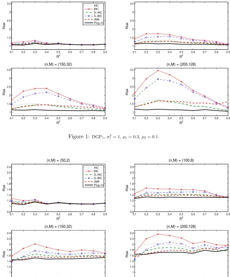
Figures 1 and 2 show the risk functions for DGP1 and DGP2 with (ρ1, ρ2) = (0.3,0.1) in the

homoskedastic simulation and Figures 3 and 4 show the risk functions for DGP1 with (ρ1, ρ2) =

(0.3,0.1) and (0.6,0.4) in the heteroskedastic simulation.1 In each figure, the risk is displayed for M = 2, 8, 32, and 128, respectively. The dotted line represents the AIC model selection estimator, the solid line with asterisk represents the BIC model selection estimator, the dash-dotted line represents the S-AIC model averaging estimator, the dash line with circle represents the S-BIC model averaging estimator, the dashed lines represents the JMA estimator, and the solid line represents the plug-in averaging estimator.

There are several remarks about the simulations results. First, the risk of all estimators in-creases as the number of models inin-creases. When we only consider the restricted and nonrestricted models, i.e. M = 2, all estimators have similar risk. Second, it can be seen that the plug-in averag-ing estimator dominates other estimators in most ranges of the populationR2. The JMA estimator has smaller risk than the S-AIC estimator for DGP2, but S-AIC achieves lower risk whenM and

R2 are larger for DGP1. The S-BIC estimator and the BIC model selection estimator have poor

performance relative to the other methods in most cases. Also note that the model-averaging-type estimators have lower risk than the model-selection-type counterpart estimators. Third, all estima-tors have smaller normalized risk under heteroskedastic errors, but the ranking of the estimaestima-tors in the heteroskedastic simulation is quite similar to that in the homoskedastic simulation. Fourth, the normalized risk of the plug-in estimator is close to 1 for DGP1, meaning that it is close to

that of the averaging estimator with infeasible optimal fixed weights. The normalized risk of the plug-in estimator is getting far from 1 as the number of models increases for DGP2. Also note that

the risk of all estimators has smaller variation across the parameters R2 in DGP2 than those in

DGP1. Fifth, as ρ1 and ρ2 increase, the risk of all estimators increases. However, the ranking of

the estimators for (ρ1, ρ2) = (0.6,0.4) is quite similar to that for (ρ1, ρ2) = (0.3,0.1).

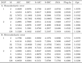
Tables 1 and 2 report the maximum risk and maximum regret of the estimators. Here we define the regret as the difference between the risk of the estimator and the optimal asymptotic risk (labeled Opt). The maximum regret is the largest value of the regret across the parameters R2_{. The maximum risk is defined as the same way. It is clear that the plug-in averaging estimator}

achieves the minimax risk and minimax regret in all simulation cases. One interesting observation from Tables 1 and 2 is that the results between DGP1and DGP2are quite different. The maximum

risk of the averaging estimator with infeasible optimal fixed weights increases as the number of models increases for DGP1, but decreases as the number of models increases for DGP2. Unlike

other estimators, the plug-in averaging estimator has relatively low maximum regret for DGP1.

Also note that the maximum risk/regert of all data-driven estimators are close to each other for DGP2. Another interesting observation is that all estimators have larger maximum risk but smaller

1

We report the results of the heteroskedastic simulations for DGP1 only for space considerations. All results are

maximum regret in the heteroskedastic simulation than in the homoskedastic simulation.

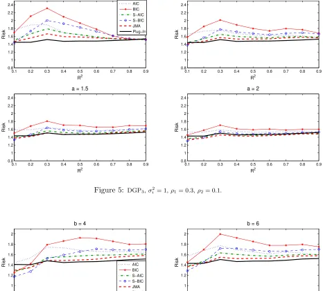
6.3 Robust Simulation

We consider two extended setups to investigate the finite sample behavior of the plug-in averag-ing estimator. The data generataverag-ing process is based on (6.1) with (ρ1, ρ2) = (0.3,0.1) and the

parameters are determined by the following:

DGP3:θ =

− √

n 8 ,

√

n 8 ,

−1,ℓ−1 ℓ , ...,−

1 ℓ

a′

c/√n, (6.4)

DGP4:θ =

− √

n b ,

√

n b ,−1,

ℓ₋1 ℓ , ...,−

1 ℓ

′

c/√n, (6.5)

where ℓ = 5, a = _{0.5,1,1.5,2_}, b = _{4,6,8,10_}, and c is selected to control the population R2_.

The sample size is 150. The number of simulations is 5000.

Figures 5 and 6 show the risk functions for DGP3 and DGP4, respectively. From Figure 5,

it can be seen that the magnitude of risk decreases as the parameter a increases. This implies that when the coefficients of auxiliary regressors decline more quickly, i.e. a is larger, the risk of all estimators are getting closer. Figure 6 shows the S-AIC, S-BIC, and JMA estimators achieves lower risk than the plug-in averaging estimator when the parameter b and R2 are small. This implies that when the auxiliary regressors have a greater influence on the model, i.e. b is larger, the plug-in averaging estimator performs better than other averaging estimators. Table 3 reports the maximum risk and maximum regret for DGP3 and DGP4. It shows that the plug-in averaging

estimator still achieves the minimax risk and minimax regret across the parameters a, b, and R2_,

even if the plug-in averaging estimator has larger risk in some ranges of the populationR2displayed in Figures 5 and 6.

7

Confidence Intervals

In this section, we propose a plug-in method to construct the confidence interval for the focus parameterµ. Sinceµis a scalar, the t-statistic is used to construct the confidence interval. Define

ˆ V =

M

X

m=1

ˆ

w_m2 Dˆ′_θmQˆ−_m1ΩˆmQˆ−m1Dˆθm+ 2

X

m<p

ˆ

wmwˆpDˆ′θmQˆ

−1

m Ωˆm,pQˆ−p1Dˆθp, (7.1)

where ˆwm could be the weight chosen by the plug-in averaging estimator, or other averaging

esti-mators with data-driven weights. The model averaging t-statistic forµ is

tn(µ) =

¯

µ(w)ˆ ₋µ

b

sen

(7.2)

Theorem 5. Suppose Assumptions 1, 3, and 4 hold. As n_{→ ∞}, we have

tn(µ)−→d (V∗)−1/2 M

X

m=1

w_m∗Λm

whereV∗=PM_m=1w∗_m2D′_θmQ−_m1ΩmQ−m1Dθm+2

P

m<pwm∗w∗pD′θmQ

−1

m Ωm,pQ−p1Dθp andΛm =a

′ mδ+

b′_mR.

Theorem 5 is a general statement for all averaging estimators with data-driven weights. For example, if weights are chosen by the plug-in averaging estimator, thenw_m∗ =w∗_pia,m, wherew∗_pia,m is defined in Theorem 2. Theorem 5 states that the asymptotic distribution of the model averaging t-statistic is not normally distributed. Instead, it is characterized by a non-linear function of the normal random vector R.

Let CIn(α) denote the 1−α percent confidence interval for parameterµwhereαis the nominal

size. By inverting the t-statistic, we construct the confidence interval with the nominal level 1₋α for the focus parameter µas CIn(α) ={µ:tn(µ)≤cn,1−α} wherecn,1−α is the critical value. The

naive way to construct the confidence interval is to use the 1₋α quantile of the standard normal distribution as the critical value. For a standard two-sided symmetric confidence interval, the naive confidence interval is defined as

CI1n(α) = [¯µ(w)ˆ −z1−α/2sebn, µ¯(w) +ˆ z1−α/2sebn] (7.3)

wherez1−α/2 is 1−α/2 quantile of the standard normal distribution. The naive confidence interval

based on normal approximations is easily to implement, but it is not a valid method since tn(µ) is

not normally distributed.

Buckland, Burnham, and Augustin (1997) propose a modified confidence interval which ad-dresses the uncertainty involved in the model selection/averaging step. They assume perfect corre-lation between any two models, which leads to a simplified formula for the variance. The confidence interval suggested by Buckland, Burnham, and Augustin (1997) is defined as

CI2n(α) = [¯µ(w)ˆ −z1−α/2seen, µ¯(w) +ˆ z1−α/2seen] (7.4)

wherese_en=PMm=1wm(˜σm2/n+ (˜µm−µ¯(w))ˆ 2)1/2 and ˜σ2m=Dˆ′θmQˆ

−1

m ΩˆmQˆ−m1Dˆθm. Here we do not need to estimate the covariance between any two submodels to calculate the standard error se_en.

However, the confidence interval proposed by Buckland, Burnham, and Augustin (1997) may still have incorrect coverage probabilities due to the non-standard distribution of the model averaging t-statistic.

and obtain the estimators δˆ, Q,ˆ Ω, andˆ Dˆθ. Second, we calculate the data-driven weights and

estimate the standard error based on (7.1). Third, we simulate the asymptotic distribution derived in Theorem 5 based on the plug-in estimators δˆ, Q,ˆ Ω, andˆ Dˆθ. Then we set the critical value

as the 1₋α quantile from the simulation. Therefore, the plug-in symmetric two-sided confidence interval is defined as

CI3n(α) = [¯µ(w)ˆ −ˆcn,1−αsebn, µ¯(w) + ˆˆ cn,1−αsebn] (7.5)

where ˆcn,1−α is the 1−α quantile of the simulated distribution.

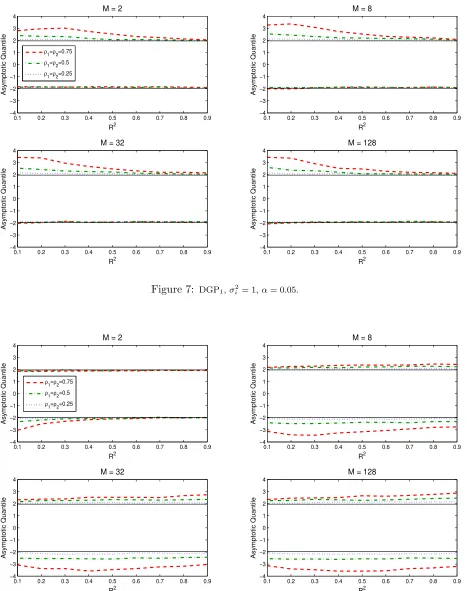
7.1 Asymptotic Quantiles

As pointed out in Theorem 5, the asymptotic distribution of the model averaging t-statistic is non-standard. Figures 7 and 8 show the quantile functions of the model averaging t-statistics for DGP1

and DGP2 under homoskedastic errors. We set α= 0.05. We simulate the asymptotic distribution

and compute the quantile function based on Theorem 5. The quantile function is approximated by using 5,000 random samples. The parameter of interest is µ= θ2 and the weights are chosen by

the plug-in averaging estimator.

In each figure, the quantile functions are displayed for M = 2, 8, 32, and 128, respectively. The dashed lines represents the quantile function for (ρ1, ρ2) = (0.75,0.75), the dash-dotted lines

represents the quantile function for (ρ1, ρ2) = (0.5,0.5), the dotted lines represents the quantile

function for (ρ1, ρ2) = (0.25,0.25), and the solid line represents the quantile function based on the

standard normal distribution.

The behavior of the quantile functions are quite similar across different number of the models. It can be seen that the asymptotic quantiles of the t-statistics are far from those of the standard normal distribution. This implies the confidence intervals using (₋1.96,1.96), the 95% quantile of the standard normal distribution, as critical points have incorrect coverage probabilities. Also note that the asymptotic quantile increases asρ1 andρ2 increase. One interesting observation from

Figures 7 and 8 is that the quantile functions are asymmetric. For DGP1, we have larger upper

critical values, while for DGP2, we have smaller lower critical values.

7.2 Coverage Probabilities

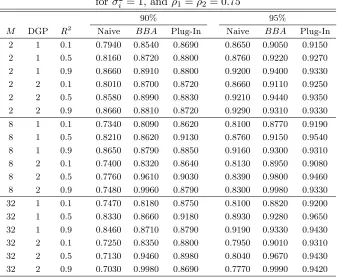
We now compare the coverage probabilities of the following methods: (1) Naive confidence interval (labeled Naive), (2) Buckland, Burnham, and Augustin (1997)’ confidence interval (labeled BBA), (3) Plug-In confidence interval (labeled Plug-In). The finite-sample coverage probabilities of the nominal 90% and 95% symmetric two-sided confidence intervals for DGP1 and DGP2 under

ho-moskedastic errors with (ρ1, ρ2) = (0.75,0.75) are reported in Table 4. The parameter of interest

isµ=θ2 and the weights are chosen by the plug-in averaging estimator. The number of repetition

As we expected, the coverage probabilities of the Naive confidence intervals are lower than the nominal level 90% and 95%. The Buckland, Burnham, and Augustin (1997)’ confidence intervals have better performance than the naive confidence intervals, however in some cases, the coverage probabilities of the Buckland, Burnham, and Augustin (1997)’ confidence intervals are larger than the nominal values. The plug-in confidence intervals have the best performance among the three methods, and the coverage probabilities of the plug-in confidence intervals are quite close to the nominal values.

8

An Empirical Example

In this section, we apply the plug-in model averaging method to cross-country growth regressions. The challenge of empirical research on economic growth is that one does not know exactly what explanatory variables should be included in the true model. Many studies attempt to identify the variables explaining the differences in growth rates across countries by regressing the average growth rate of GDP per capita on a large set of potentially relevant variables, see Durlauf, Johnson, and Temple (2005) for a literature review. Due to the limited number of the observations and a large amount of the candidate variables, the empirical growth literature has been heavily criticized for its kitchen-sink approach.

In order to take into account the model uncertainty, Bayesian model averaging techniques have been applied to empirical growth, including Fernandez, Ley, and Steel (2001), Sala-i Martin, Doppelhofer, and Miller (2004), Durlauf, Kourtellos, and Tan (2008), and Magnus, Powell, and Prufer (2010). We apply frequentist model averaging approaches as an alternative to Bayesian model averaging techniques to economic growth. We estimate the following cross-country growth regression

gi =x′iβ+z′iγ+ei (8.1)

where gi is average growth rate of GDP per capita between 1960 and 1996, xi are the Solow

variables from the neoclassical growth theory, and zi are fundamental growth determinants such

as geography, institutions, religion, and ethnic fractionalization from the new fundamental growth theory. Here, xi are core regressors which appear in every submodels, while zi are the auxiliary

regressors which serve as controls of the neoclassical growth theory and may or may not be included in the submodels.

fraction of Confucian population (CONFUC), see Magnus, Powell, and Prufer (2010) for a detailed description of the data. Model Setup B contains only one core regressor, the constant term, and all other variables in Model Setup A are auxiliary regressors. The parameter of interest is the convergence term of the Solow growth model, that is, the coefficient of the log GDP per capita in 1960. The total number of observations is 74. We consider all possible submodels, that is, we have 16 submodels in Model Setup A and 512 submodels in Model Setup B.

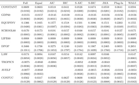
We consider eight estimators: (1) the least-squares estimator for the full model (Full), (2) the averaging estimator with equal weights (Equal), (3) AIC model selection estimator (AIC), (4) BIC model selection estimator (BIC), (5) S-AIC model averaging estimator (S-AIC), (6) S-BIC model averaging estimator (S-BIC), (7) Jackknife Model Averaging estimator (JMA), and (8) Plug-In averaging estimator (Plug-In). The standard errors of data-driven model averaging estimators are calculated by (7.1).

The estimation results for Model Setup A and B are given in Table 5 and 6, respectively. We also repot the estimation results for weighted-average least-squares (WALS) estimator proposed by Magnus, Powell, and Prufer (2010) for comparison. The WALS estimator is a Bayesian model averaging technique which uses a Laplace distribution instead of the normal prior as the parameter prior. The results in Table 5 and 6 show that all coefficients have the same signs across different estimation methods. In model A, the coefficient estimate and standard error of GDP60 are similar between Plug-In, Full, Equal, and JMA estimators. Also, the 90% plug-in confidence interval for GDP60 is (₋0.0206,₋0.0107), which is close to the naive confidence interval (₋0.0200,₋0.0112).

In Model Setup B, the plug-in averaging estimate of GDP60 is quite close to the least-squares estimate from the full model and is higher in absolute value than other estimates. The 90% plug-in confidence interval for GDP60 is (₋0.0205,₋0.0102), which is wider than the naive confidence inter-val (₋0.0183,₋0.0124). The equal-weight averaging estimator has the smallest coefficient estimate and standard error of GDP60 because only half of submodels contains the regressor GDP60. The important finding from our results is that the plug-in averaging estimator has the smaller standard error of GDP60 than other estimators, except for the averaging estimator with equal weights.

It is also instructive to contrast the results of the Plug-In and WALS estimators. In Model Setup A, the estimation results are similar between Plug-In and WALS. In Model Setup B, the estimated coefficient of GDP60 is higher in absolute value for Plug-In than for WALS, while the estimated standard error of GDP60 is much smaller for Plug-In than for WALS. Therefore, the convergence speed of the growth model implied by our result is higher than that found by Magnus, Powell, and Prufer (2010). Comparing the results between Model Setup A and Model Setup B, we find that the plug-in averaging estimator chooses different fundamental growth determinants in different model specifications. Therefore, our results support the findings of Durlauf, Kourtellos, and Tan (2008) and Magnus, Powell, and Prufer (2010) that the fundamental variables are not robustly correlated with growth.

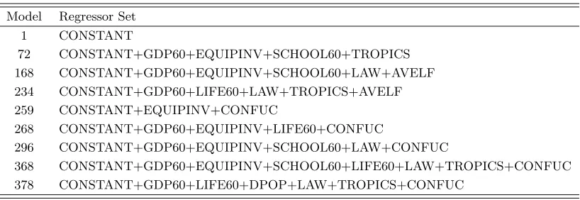
Table 7-10 we can see that AIC chooses a larger model than BIC in both model specifications, which is consistent with the previous literature. One interesting observation is that JMA and Plug-In choose completely different submodels in Model Setup A and B. The submodels chosen by JMA cover all entire regressor set, while Plug-In excludes the regressors LAW and TROPICS in Model Setup A and the regressors EQUIPINV, SCHOOL60, DPOP, and CONFUC in Model Setup B. Note that Plug-In puts 30% weight on the smallest submodel in Model Setup B. This particular model choice can explain the relatively small standard error of GDP60 of the plug-in estimate.

9

Conclusion

Appendix

A

Proofs

Proof of Lemma 1: We first show the asymptotic distribution of the least-squares estimator for the full model. By Assumption 2 and the application of the continuous mapping theorem, it follows that

√

nθˆ₋θ=

1 nH

′_H

−1 ₁

√

nH

′_e

d

−→Q−1R_∼N(0,Q−1ΩQ−1).

We next show the asymptotic distribution of the least-squares estimator for each submodel. Define the extended selection matrixSm as

Sm =

Ik 0k×ℓm 0ℓ×k Π′m

!

.

Then we have Hm = (X,ZΠ′m) =HSm and Ωm=S′mΩSm. By some algebra, it follows that

˜

θm= (H′mHm)−1H′my

= H′_mHm−1 H′m Xβ+ZΠm′ Πmγ+Z(Iℓ−Π′mΠm)γ+e

= H′_mHm−1H′mHmθm+ H′mHm−1H′mZ Iℓ−Π′mΠmγ+ H′mHm−1H′me

=θm+ H′mHm−1H′mZ Iℓ−Πm′ Πmγ+ H′mHm−1S′mH′e.

Therefore, by Assumptions 1-2 and the application of the continuous mapping theorem, we have

√

nθ˜m−θm

=

1 nH

′ mHm

−1

1 nH

′ mZ

I_ℓ−Π′_mΠm√nγ+

1 nH

′ mHm

−1

S′_m

1

√

nH

′_e

d

−→Q−_m1 Qxz ΠmQzz

!

Iℓ−Π′mΠmδ+Q−m1S′mR

=Amδ+BmR∼N Amδ, Q−m1ΩmQ−m1

where

Am =Q−m1

Qxz ΠmQzz

!

Iℓ−Π′mΠm and Bm=Q−m1S′m.

This completes the proof.

Proof of Lemma 2: Define γ_mc ={γ :γ_j ∈/ γ_m, f or j = 1, ..., ℓ}. That is, γ_mc is the set of parameters γj which are not included in submodelm. Hence, we can writeµ(θ) as µ(β,γm,γmc). Also,µ(θm) =µ(β,γm,0).

Note that γ=O(n−1/2) by Assumption 1. Then by a standard Taylor series expansion ofµ(θ) about γmc =0, it follows that

µ(β,γm,γmc) =µ(β,γ_m,0) +D′_γ

mcγmc+O(n

−1₎

That is, µ(θ)₋µ(θ_m) =D′γ(Iℓ−Π′mΠm)γ+O(n−1). Thus, by Assumptions 1-2 and the

appli-cation of the delta method, we have

√

nµ(θ˜m)−µ(θ)

=√nµ(θ˜m)−µ(θm)

−√nµ(θ)₋µ(θm)

d

−→D′_θm(Amδ+BmR)−D′γ Iℓ−Π′mΠmδ

=D′_θmAmδ−D′γ Iℓ−Π′mΠmδ+D′θmBmR = D′_θmQ−_m1 Qxz

ΠmQzz

!

−D′_γ

!

Iℓ−Π′mΠmδ+D′θmQ

−1

m S′mR

=a′_mδ+b′_mR_≡Λm∼N a′mδ, D′θmQ

−1

m ΩmQ−m1Dθm

,

where

am= Iℓ−Π′mΠm

Qzx QzzΠ′_m

!

Q−_m1Dθm−Dγ

!

,

bm=SmQ−m1Dθm.

This completes the proof.

Proof of Theorem 1: From Lemma 2, there is joint convergence in distribution of all

√

nµ(θ˜_m)₋µ(θ) to Λm since all of Λm can be expressed in terms of R. Since the weights

are non-random, it follows that

√

n(¯µ(w)₋µ) =

M

X

m=1

wm√n(˜µm−µ)−→d M

X

m=1

wmΛm ≡Λ.

Therefore, the asymptotic distribution of the averaging estimator is a weighted average of the normal distributions which is also a normal distribution.

By Lemma 2 and standard algebra, we can show the mean of Λ as

E

M

X

m=1

wmΛm

!

=

M

X

m=1

wmE (Λm) = M

X

m=1

wma′mδ=a′δ, anda= M

X

m=1

wmam.

Next we want to show the variance of Λ. For any two submodels, we have

Cov(Λm,Λp) = E a′mδ+b′mR−E(a′mδ+b′mR)

a′_pδ+b′_pR₋E(a′_pδ+b′_pR) = E b′_mRb′_pR

=b′_mE RR′bp

=D′_θmQ−_m1S′_mΩSpQ−p1Dθp

=D′_θmQ−_m1Ωm,pQ−p1Dθp

with

Ωm,p =

Ωxx ΩxzΠ

′ p

ΠmΩzx ΠmΩzzΠ′_p

where the second equality holds by the fact that am, bm, and δ are constant vectors and R ∼

N(0,Ω). Therefore, variance of Λ is

V =var

M

X

m=1

wmΛm

!

=

M

X

m=1

w2_mV ar(Λm) + 2

X

m<p

wmwpCov(Λm,Λp)

=

M

X

m=1

w2_mD′_θmQ_m−1ΩmQ−m1Dθm+ 2

X

m<p

wmwpD′θmQ

−1

m Ωm,pQ−p1Dθp.

This completes the proof.

Proof of Theorem 2: We first show Dˆθm, Qˆm, Ωˆm,p, and ˆam are consistent estimators for Dθm, Qm, Ωm,p, and am. By Lemma 1, we have θˆ

p

−→ θ, which also implies that ∂µ(θˆ)/∂θ = ˆ

Dθ

p

−→Dθ. By Assumption 2 and 3 and the fact that the selection matrix is non-random, we have

ˆ Dθm

p

−→ Dθm, Qˆm

p

−→ Qm, and Ωˆm,p p

−→ Ωm,p. By Assumption 2 and the application of the

continuous mapping theorem, it follows that ˆam −→p am.

We next show the limiting distribution of ˆζm,p. By Assumption 2 and 3 and the application of

the continuous mapping theorem, it follows thatDˆ′_θ m

ˆ

Q−_m1Ωˆm,pQˆ−p1Dˆθp

p −→D′_θ

mQ

−1

m Ωm,pQ−p1Dθp. Recall that δˆ_−→d Rδ =δ+ΠℓQ−1R. Then by the application of Slutsky’s theorem, we have

ˆ

ζm,p=δˆ′ˆamˆa′pδˆ+Dˆ′θmQˆ

−1

m Ωˆm,pQˆ−p1Dˆθp

d

−→R′_δamap′Rδ+D′θmQ

−1

mΩm,pQ−p1Dθp =ζ

∗ m,p.

Since all of ζ_m,p∗ can be expressed in terms of the normal random vector R, there is joint

convergence in distribution of all ˆζm,p to ζm,p∗ . Hence, it follows thatw′ζˆw d

−→w′ζ∗w.

We now show the limiting distribution of wˆpia. Note that w′ζ∗w is a convex minimization

problem sincew′ζ∗wis quadratic andζ∗ is positive definite. Hence, the limiting processw′ζ∗wis continuous in w and has a unique minimum. Also note that wˆpia = Op(1). By Theorem 3.2.2 of

Van der Vaart and Wellner (1996) or Theorem 2.7 of Kim and Pollard (1990), the minimizerwˆpia

converges in distribution to the minimizer of w′ζ∗w, which isw_pia∗ .

Finally, we show the asymptotic distribution of the plug-in averaging estimator. Since both Λm and w∗pia,m can be expressed in terms of the same normal random vector R, there is joint

convergence in distribution of all ˜µm and ˆwpia,m. By Lemma 2, (4.2), and (4.9), it follows that

√

n µ¯(wˆpia)−µ= M

X

m=1

ˆ

wpia,m√n(˜µm−µ)−→d M

X

m=1

w_pia,m∗ Λm.

This completes the proof.

Proof of Theorem 3: By (5.2) and (5.3), it follows that ˆwsaic,m −→d w∗saic,m. Also, there

is joint convergence in distribution of all ˆwwsaic,m and ˜µm. Thus, the limiting distribution of the

Proof of Theorem 4: Define hi =h′i(H′H)−1hi. Notice that ˆe−i = ˆei(1−hi)−1≈ˆei(1 +hi)

where ˆeiis the least-squares residuals and ˆe−iis the leave-one-out least-squares residual from the full

model. For the submodel m, we have hm,i = (x′i,z′iΠm)′ = (x′i,z′mi)′,hm,i =h′m,i(H′mHm)−1hm,i,

and ˜em,−i ≈e˜m,i(1 +hm,i).

Then it follows that

1 n n X i=1 ˜

em,−ie˜p,−i ≈

1 n n X i=1 ˜

em,ie˜p,i+

1 n n X i=1 ˜

em,i˜ep,i(hm,i+hp,i) +

1 n n X i=1 ˜

em,i˜ep,ihm,ihp,i

= 1 n n X i=1 ˜

em,ie˜p,i+

1 n n X i=1 ˜

em,i˜ep,ih′m,i H′mHm−1hm,i

+ 1 n n X i=1 ˜

em,i˜ep,ih′p,i Hp′Hp−1hp,i+o(1)

= 1 n n X i=1 ˜

em,ie˜p,i+

1

ntr H

′

mHm−1 n

X

i=1

hm,ih′m,i˜em,ie˜p,i

!

+ 1

ntr H

′ pHp−1

n

X

i=1

hp,ih′p,ie˜m,i˜ep,i

!

+o(1)

= 1 n n X i=1 ˜

em,ie˜p,i+ 1

ntr

ˆ

Q−_m1Ω˜m,m,p

+ 1 ntr

ˆ

Q−_p1Ω˜p,m,p

+o(1),

where

ˆ Qm=

1 n n X i=1 xi zmi !

x′_i z′_mi ,

˜

Ωm,m,p= 1

n n X i=1 xi zmi !

x′_i z′_mi e˜m,i˜ep,i.

Therefore, we have

ξm,p=˜e′m,−i˜ep,−i−ˆe′ˆe

= ˜e′_m˜ep−ˆe′ˆe+tr

ˆ

Q−_m1Ω˜m,m,p

+trQˆ−_p1Ω˜p,m,p

+o(1), (A.1)

whereˆe=y₋H ˆθ and˜em =y−Hmθ˜m.

First, we consider the first terms of (A.1). Since ˜e′_mˆe=ˆe′ˆeand ˜em−ˆe =H(Smθ˜m−θˆ), we

have

˜e′_m˜ep−ˆe′ˆe= (˜em−ˆe)′(˜ep−ˆe)

=√n(θˆ₋Smθ˜m)′

1 nH

′_H√_n(θˆ

Define Πℓ= (0ℓ×k,Iℓ). Then from Lemma 1 it follows that √

n(θˆ₋Smθ˜m) =√n(θˆ−θ)−Sm√n(θ˜m−θm) +√n(θ−Smθm)

d

−→Q−1R₋Sm Q−m1

Qxz ΠmQzz

!

Iℓ−Π′mΠmδ+Q−m1S′mR

!

+ 0k×1 (Iℓ−Π′mΠm)δ

!

= Q−1₋SmQ−m1S′m

R+ Π′_ℓ−SmQ−m1

Qxz ΠmQzz

!!

Iℓ−Π′mΠmδ

=A¨mδ+B¨mR≡R¨m

where

¨

Am= Π′ℓ−SmQ−m1

Qxz ΠmQzz

!!

Iℓ−Π′mΠm, and B¨m = Q−1−SmQ−m1S′m

.

Therefore, it follows that

˜

e′_m˜ep−ˆe′eˆ−→d R¨′mQ ¨Rp. (A.2)

Next, consider the second and third terms of (A.1). From Lemma 3 and the application of the continuous mapping theorem, it follows that

tr(Qˆ−_m1Ω˜m,m,p) p

−→tr(Q−_m1Ωm), (A.3)

tr(Qˆ−_p1Ω˜p,m,p) p

−→tr(Q−_p1Ωp), (A.4)

Equation (5.9) then follows from (A.2), (A.3), and (A.4). Since all of ξ∗_m,p can be expressed in terms of the normal random vector R, there is joint convergence in distribution of allξm,p toξ∗m,p.

Hence, it follows that w′ξnw−→d w′ξ∗w.

Finally, we show the limiting distribution of wˆjma and ¯µ(wˆjma). First, the limiting process

w′ξ∗wis continuous in wand has a unique minimum sincew′ξ∗w is quadratic and ξ∗ is positive definite. Second, wˆjma = Op(1) by the fact that Hn is convex. Therefore, by Theorem 3.2.2 of

Van der Vaart and Wellner (1996) or Theorem 2.7 of Kim and Pollard (1990), the minimizerwˆjma

converges in distribution to the minimizer of w′ξ∗w, which is w_jma∗ . Equation (5.11) then follows from the distribution result (5.10) and the fact that there is joint convergence in distribution of ˜µm

and wˆjma. This completes the proof.

Lemma 3. Let e˜m,i=yi−xi′βˆm−z′miγˆm denote the OLS residuals from the submodels and

˜

Ωm,m,p=

1 n

n

X

i=1

xi

zmi

!

x′_i z′_mi e˜m,i˜ep,i

for m, p= 1, ..., M. Suppose Assumptions 1 and 4 hold. As n_{→ ∞}, we have

˜ Ωm,m,p