Bayesian Portfolio Selection in a Markov Switching Gaussian Mixture Model

Munich Personal RePEc Archive

Bayesian Portfolio Selection in a Markov

Switching Gaussian Mixture Model

Qian, Hang

Iowa State University

24 December 2011

Online at

https://mpra.ub.uni-muenchen.de/35561/

Bayesian Portfolio Selection in a Markov Switching

Gaussian Mixture Model

Hang Qian1

Abstract

Departure from normality poses implementation barriers to the Markowitz

mean-variance portfolio selection. When assets are affected by common and

idiosyncratic shocks, the distribution of asset returns may exhibit Markov

switching regimes and have a Gaussian mixture distribution conditional on

each regime. The model is estimated in a Bayesian framework using the

Gibbs sampler. An application to the global portfolio diversification is also

discussed.

Keywords: Portfolio, Bayesian, Hidden Markov Model, Gaussian Mixture.

1. Introduction

Markowitz (1952) mean-variance analysis is consistent with an investor’s

utility maximization when the asset returns are normally distributed.

How-ever, it has long been recognized by practitioners and scholars that financial

asset returns often depart from normality. Investors usually feel that the

stock prices crawl upwards for months but plummet in a day, which is hard

to reconcile with the relative thin and symmetric tail of a normal

distribu-1_{Corresponding author: Department of Economics, Iowa State University, Ames, IA,}

tion. There is abundant of empirical evidence suggesting unconditional asset

returns exhibit skewness, fat fail and extreme values (e.g., Fama, 1965;

Blat-tberg and Gonedes, 1974; Peiro, 1999; Ane and Geman, 2000, to name a few).

In that case, the mean and variance are inadequate to characterize all the

rel-evant aspects of the optimal portfolio. Higher order moments will play a role

in the portfolio selection and asset pricing. From a theoretical perspective,

Kraus and Litzenberger (1976) model the skewness preference and its effect

on risk assets valuation. Harvey and Siddique (2000) empirically test the

effect of conditional skewness on the asset pricing. Jondeau and Rockinger

(2006) use a fourth order Taylor expansion of the expected utility to quantify

the extent to which non-normality affects the optimal asset allocation.

Given the stylized fact of departure from normality, it is natural to

pro-pose some other distributions that can better accommodate skewness,

lep-tokurtosis and extreme values. Some early works use symmetric stable

dis-tribution (Fama, 1965) and Student-t disdis-tribution (Blattberg and Gonedes,

1974) to account for the fat tail but not skewness. Harvey et al. (2010)

consider the portfolio selection with a multivariate skew normal distribution,

which allows skewness and coskewness. A skew normal random variable is

essentially the sum of a normal and half normal variate. It is not easy to

pro-vide an economic interpretation of the half normal variate, since the sum of

two half normal is no longer half normal. Modeling asset returns with skew

normal distribution is largely an empirical strategy that conveniently and

effectively addresses the concern of skewed returns. Buckley et al. (2008) use

the Gaussian mixture distribution in the portfolio optimization. Gaussian

mar-ket regimes. Furthermore, Gaussian mixture can mimic many complicated

distribution. For instance, if we assign a large probability to the first regime

and a low probability to the second regime with a large mean and large

vari-ance, the mixture is similar to a positively skewed distribution. If the second

regime has a large mean and small variance, the mixture is close to a

nor-mal distribution with occasional extreme values. If we mix infinite number

of normal distributions with the same mean and inverse-gamma distributed

variances, the mixture is a Student t distribution that allows leptokurtosis.

In the Gaussian mixture, the latent regimes are random draws from a

multinomial distribution without autocorrelation. As a generalization, if the

latent regimes are allowed to have a Markov law of motion, the mixture

be-comes a hidden Markov model (HMM) initially proposed by Baum and his

colleagues (Baum and Petrie, 1966; Baum and Eagon, 1967; Baum et al.,

1970). It has been successfully applied to a variety of fields such as speech

recognition, signal process (Rabiner, 1989). This model is mostly known to

economists in another name: the Markov (regime) switching model.

Hamil-ton (1989) models the mean GNP growth rate with two Markov switching

regimes. Turner et al. (1989) consider the variance of a portfolio’s excess

returns depends on a Markov switching state variable. There are many

sub-sequent works that extend the Markov switching model to vector

autore-gression (Krolzig, 1997), endogenous regime transition (Kim et al., 2008),

etc.

In this paper, we consider a scenario that asset prices are affected by two

types of latent shocks. The first type is common shocks on all assets, which

each individual asset, which lead to a Gaussian mixture returns with different

states. The joint forces of the common and idiosyncratic shocks make asset

returns follow a Markov switching Gaussian mixture (MSGM) distribution.

It is possible to write down the likelihood function of our model in a

recursive manner, and then estimate the model by maximum likelihood or

E-M algorithm. However, when the number of regimes/states become

mod-erately large, say more than three, the model contains many parameters and

the numerical maximization can hardly perform satisfactorily in practice. 2

Roman et al. (2010) conclude that “although theoretically the HMM-based

time series modeling can tackle the multivariate case, from a practical point

of view it has limited applicability”. Our model is estimated in a Bayesian

framework. Given an appropriate estimation routine, it can reliably

esti-mate model for moderately large number of regimes/states with affordable

2_{There are many available estimation routines of Markov switching model. On his}

web-site, Professor James Hamilton collects links to these programs. A well-received MATLAB

program by Marcelo Perlin estimates the model by direct maximization of the log

likeli-hood. In the manual, Marcelo advises against the use of the model with more than three

regimes. He mentions “the solution is probably a local maximum and you can’t really trust

the output you get”. In the MATLAB statistic toolbox there is a routine “hmmtrain.m”for

estimating discrete HMM model by the E-M algorithm. However, we test the routine with

three or four regimes using pseudo data with known data generating process, the program

cannot reliably estimate the model if the initial values are not carefully chosen. In a

tuto-rial to regime-switching models, Hamilton (2005) mentions most applications assume two

or three regimes and “there is considerable promise in models with a much larger number

of regimes, either by tightly parameterizing the relation between the regimes (Calvet and

computation costs.

Estimating our model in the Bayesian framework has another

advan-tage. The classic Markowitz portfolio selection has an implementation

bar-rier called the “estimation risk”, that is, our inability to provide the exact

inputs since the population mean and covariance matrix of asset returns are

unknown. One might resort to the sample analog as a certainty equivalent

so-lution. It is well documented that the portfolio weights under that approach

tend to be volatile, sensitive to minor inputs change and lack

diversifica-tion (Dickinson, 1974; Jobson and Korkie, 1980; Black and Litterman, 1992;

Michaud and Michaud, 2008, among others). The instability of portfolio

weights is believed to be caused by the negligence of parameter uncertainty,

especially the estimation error of the mean. Chopra and Ziemba (1993) find

that error in means is ten-fold as devastating as errors in variances.

Further-more, assets with high sample average return and low sample variance will

be assigned larger weight in the portfolio, but those asset returns are more

likely to be error-ridden (Scherer, 2002). In the Bayesian framework, the

problem of the estimation risk is resolved since our triple uncertainties over

the regimes/states, parameters and future disturbances are fully embodied

in the posterior predictive distribution.

The rest of the paper is organized as follows. Section 2 lays out a

micro-foundation that the assets prices and returns follow the MSGM distribution

when the assets are subject to common and idiosyncratic shocks. Section 3

outlines the econometric model and the Gibbs sampler to obtain posterior

draws of model parameters as well as hidden regimes and states. Section 4

asset returns. Section 5 provides an illustrative application and compares

performance our model to the classic portfolio selection model. Section 6

concludes the paper.

2. Micro Foundation

Though our asset returns model is primarily an empirical econometric

model that flexibly accommodates non-normality, it has a micro foundation.

The hidden Markov Gaussian mixture asset returns can be justified by a

Lucas asset-pricing model (Lucas, 1978), where we slightly adapt the classic

model by decomposing the exogenous productivity shocks into common and

idiosyncratic components. The former induces Markov switching regimes and

the latter leads to mixture normal returns conditional on a regime.

Consider a pure exchange economy consisting of numerous identical agents

with n varieties of fruit trees that are symbolic of assets. Normalize the

number of agents and trees of each variety to one. At the beginning of a

pe-riod, trees yield stochastic fruits, a parable of exogenous productivity shocks.

Then agents eat fruits and trade trees at market prices. Assume logarithmic

preferences, the sequential optimization problem of an agent is formulated as

max

{Ci,t,Ai,t}

E0

" _∞ X

t=0

n X

i=1

βtlnCi,t #

,

n X

i=1

(Ci,t+pi,tAi,t+1) =

n X

i=1

(pi,tAi,t+di,tAi,t) ,

wheredi,t is the yield of fruiti in periodt. At the market pricepi,t, an agent

that exogenous productivity shocks are mainly determined by the weather

dummy wt and vermin dummy vi,t in a regression style:

lndi,t =αi+γi ·wt+δi·vi,t+εi,t.

The baseline yield of fruitiis exp (αi). The period-tweather conditionwt

simultaneously affects trees of all varieties, though with varied magnitudes

on different fruits. Assumewtfollows a Markov chain with two regimes. The

weather condition is symbolic of common shocks in the macroeconomy that

affect all financial assets. As the weather can be “sun” or “rain”, the market

can be heuristically labeled as “bull” or “bear”. On the other hand, trees may

be also subject to vermin intrusion and assume each variety of fruit tree is

vulnerable to a species of worm, captured by the dummy variablevi,t for fruit

i in period t. The presence of vermin is a metaphor of major idiosyncratic

shocks to a financial asset. Lastly, the disturbance εi,t captures countless

minor common or idiosyncratic factors that may affect fruits harvest. Assume

(ε1,t, ..., εn,t|wt =s)∼N(0,Σs),s = 1,2.

The solution to the Lucas tree model is standard. By iterating forward

the Euler equation

pi,t =Et

β Ci,t Ci,t+1

(pi,t+1+di,t+1)

,i= 1, ..., n,t _≥0,

we obtain the fundamental asset price without bubbles

pi,t =Et " _∞

X

j=1

βj Ci,t

Ci,t+j

di,t+j #

.

On the other hand, the market clearing condition requires Ci,t+j = di,t+j,

∀j _≥0. So the asset pricing equation is eventually given by

pi,t =

β

or

lnpi,t = [lnβ−ln (1−β) +αi] +γiwt+δivi,t+εi,t.

The asset return from period t ₋ 1 to t consists of capital gains and

dividend income, which can be thought as the log difference of the

dividend-adjusted price series.

ri,t ≡ln (pi,t+di,t)−lnpi,t−1

=₋lnβ+γi(wt−wt−1) +δi(vi,t−vi,t−1) + (εi,t−εi,t−1)

Typically a researcher observes neither common nor idiosyncratic shocks,

therefore we marginalize lnpi,t and ri,t with respect to wt, vi,t. First

con-sider the distribution of logarithmic asset prices. (lnp1,t, ...,lnpn,t) follows

a two-regime hidden Markov chain. Conditional on each regime, there are

2n _{latent states determined by idiosyncratic shocks. Further conditional on}

each state, it follows a multivariate normal distribution. In other words, the

distribution of logarithmic asset prices is a hidden Markov Gaussian mixture.

Next consider the distribution of asset returns. Put the weather conditions

in periodt and period t₋1 as a pair, the joint returns (r1,t, ..., rn,t) follows a

four-regime hidden Markov chain. Conditional on each regime, it is a

Gaus-sian mixture with 4n _{latent states. Therefore, the Lucas tree model justifies}

both logarithmic asset prices and returns follow the MSGM distribution.

3. Econometric Model

In this section, we build an econometric model of asset prices

Let the returns of n assets be Yt = (r1,t, ..., rn,t)′, t = 1, ..., T. Denote

YT₁ =_{Yt}T_t=1.Assume assets returns are driven by a hidden Markov chain

with S regimes. Let the latent regime in period t be τt ∈ {1, ..., S} and

denote τT

1 = {τt}T_t=1. The initial (period 1) distribution is π = (π1, ..., πS)′

and the transition matrix is given by

Q=      Q1 ... QS     =     

Q1,1 ... Q1,S

...

QS,1 ... QS,S     .

Conditional on τt, Yt follow a Gaussian mixture with K latent states.

Let the latent states be λt∈ {1, ..., K}, following a multinomial distribution

with probabilityηs= (ηs,1, ..., ηs,K)′ under the current regimes. Ifτt, λtwere

known, Yt would be a multivariate normal vector.

P (Yt|τt, λt) = S Y s=1 K Y k=1

[φ(Yt;µs,k,Σs,k)]

I(τt=s)·I(λt=k)_,

where φ(_·) is the density of a multivariate normal distribution, and I(_·) is

an indicator function that takes one if the expression in the parenthesis is

true and takes zero otherwise. Note that the theoretic model in Section 2

suggests the covariance matrix Σs,k does not change with the latent statek.

This restriction can greatly reduce the number of parameters in the model,

though as a general econometric model we allow the covariance matrix to

Conjugate proper priors of model parameters are specified as

µs,k ∼N(bs,k,Vs,k) ,

(Σs,k)−1 ∼W hishart(Ωs,k, νs,k) ,

Qs ∼Dirichlet(as,1, ..., as,S) ,

π ∼Dirichlet(c1, ..., cS) ,

ηs ∼Dirichlet(fs,1, ..., fs,K) ,

wheres = 1, ..., S and k = 1, ..., K.

The full posterior conditional distribution of µs,k is given by

µs,k|· ∼N(Ds,kds,k,Ds,k) ,

where

Ds,k =

Ts,k(Σs,k)−1+ (Vs,k)−1 −1

,

ds,k = (Σs,k)−1 T X

t=1

[Yt·I(τt=s, λt =k)] + (Vs,k)−1bs,k,

Ts,k = T X

t=1

I(τt =s, λt=k) .

In other words, the posterior µs,k is determined by its prior as well as

observations that fall into regimes and statek. Similarly, the posteriorΣs,k

is determined by its prior as well as observations that fall into the regime s

and the state k. It follows that

(Σs,k)−1|· ∼W hishart Ωs,k, νs,k

where

Ωs,k = (

(Ωs,k)−1+ T X

t=1

(Yt−µs,k) (Yt−µs,k)′·I(τt=s, λt =k) )−1

,

νs,k =νs,k+Ts,k.

In models where Σs,k does not vary with the state k, the posterior Σs,k

takes a similar form by replacingI(τt=s, λt =k) with I(τt =s) during the

summation. If Σs,k further does not change with regimes, the summation is

taken for the whole sample period.

The posterior of the mixture probability is given by

ηs|· ∼Dirichlet(fs,1+Ts,1, ..., fs,K +Ts,K) .

The posterior λt can take one of the K discrete states. The posterior

distribution takes the form

P (λt=k|·)∝ S Y

s=1

[ηs,kφ(Yt;µs,k,Σs,k)]

I(τt=s)_,

where k = 1, ...K. It follows that λt = k|· has a multinomial distribution

with probability proportional to

S Y

s=1

[ηs,kφ(Yt;µs,k,Σs,k)]I(τt=s).

The posterior of the initial distribution of the Markov chain is

π_|· ∼Dirichlet[c1+I(τ1 = 1), ..., cS+I(τ1 =S)] .

The posterior of the transition matrix of the Markov chain takes the form

Qs|· ∼Dirichlet

h

as,1+Tes,1, ..., as,S +Tes,S i

,

where Tes,j = PT

The posterior latent regimesτt can take one of the S discrete regimes. A

straightforward method of sampling τt is to make use of its two neighbors

τt−1 and τt+1. However, MCMC chain may mix poorly due to excessive

nodes on the chain. A better method is to sample the entire series τT

1 by

the Baum-Welch algorithm. The algorithm outlined here is similar to Chib

(1996), who uses a backward induction. We sample the latent regimes in a

forward sequence: τ1, τ2, τ3, etc.

Letθ be all the parameters of the model (includingµs,k,Σs,k,ηs, Qs, π).

Define the forward variable

Ft,s=P τt=s,Yt1

θ,λT

1

, t= 1, ..., T, s = 1, ..., S.

The forward variable can be computed by forward induction:

Ft,s = " _K

Y

k=1

φ(Yt;µs,k,Σs,k)I(λt=k) #

·

S X

r=1

Ft−1,rQr,s,

Similarly define the backward variable

Bt,s =P YTt+1

θ, λT

1, τt =s

,

which can be computed by backward induction:

Bt,s = S X

r=1

Qs,r· " _K

Y

k=1

φ(Yt+1;µr,k,Σr,k)

I(λt+1=k)

#

·Bt+1,r,

Note thatP τT

1

YT₁, θ, λT

1

=P τ1

Y₁T, θ, λT

1 · T Y t=2

P τt

τt−1,Y1T, θ, λT1

,

so we sample τT

1 by the method of composition.

For each s, r= 1, ..., S, we have

P τ1 =s

YT₁, θ ∝F1,s·B1,s,

P τt=s

τt−1 =r,YT1, θ

∝Qr,s· " _K

Y

k=1

φ(Yt;µs,k,Σs,k) I(λt=k)

#

The sampler for the latent regimes can be further improved by using the

Gaussian mixture instead of normal distribution. Note that in the above

procedure, τT

1 is sampled from its full posterior conditionals, in which we

explore the realization of the latent states λt in the mixture so that the

term

K Y

k=1

φ(Yt;µs,k,Σs,k) I(λt=k)

is effectively a normal density. However, if

we put τT

1 and λT1 in a block and sample them together using the method of

composition, the nodes on the MCMC will be shortened and mixing property

can be improved. In the block sampler, we first sample τT

1 from it posterior

distribution without being conditional on λT

1, then we sample λT1 from its

full posterior conditionals. The previous procedure is modified by

Ft,s= " _K

X

k=1

ηs,kφ(Yt;µs,k,Σs,k) #

·

S X

r=1

Ft−1,rQr,s,

Bt,s= S X

r=1

Qs,r· " _K

X

k=1

ηr,kφ(Yt+1;µr,k,Σr,k) #

·Bt+1,r,

and

P τt=s

τt−1 =r,Y1T, θ

∝Qr,s· " _K

X

k=1

ηs,kφ(Yt;µs,k,Σs,k) #

·Bt,s.

There is a note to the above Gibbs sampler. The hidden Markov models

and Gaussian mixture models have an identification problem, that is, the

likelihood function is invariant to regime/state label switching. There are

some controversies over the interpretation of the label switching problem.

Celeux et al. (2000) argue that virtually the entirety of MCMC samplers to

the mixture model fails to converge due to the computational and inferential

difficulties. Jasra et al. (2005) pessimistically believe that Gibbs sampler

battle, Fruhwirth-Schnatter (2001) addresses the problem directly by adding

a parameter random permutation step after each iteration of the

simula-tor. Geweke (2007) insightfully points out that Gibbs sampler can reliably

recover the posterior as long as the function of interest is invariant to

per-mutation. He also proposes a conceptual permutation-augmented posterior

simulator. Our function of interest is the posterior predictive asset returns

whose distribution does not depend on the regime/state label. So the labeling

phenomenon is not a problem.

4. Investor’s Problem

Once we have a probability model on the asset returns, we are ready

to solve an investor’s portfolio optimization problem. It is most natural

to assume the goal of portfolio selection is to maximize expected utility on

future portfolio returns, though there are other ways to define the goal of

portfolio optimization. For example, Buckley et al. (2008) consider

maxi-mizing the portfolio Sharpe ratio and out-performance probability of return

target. When the asset returns are normally distributed, these goals are

closed related and consistent with each other. However, different goals lead

to different portfolios when asset returns depart from normality. In this

sec-tion, we discuss an investor’s problem in the expected utility maximization

framework.

Let u(_·) be a standard utility function. Assume the investor maximizes

expected returns Eu(ω′YT+1)

YT

1

subject to ω′ι = 1, where ω is the

portfolio weights and ι is a vector of ones.3

With MCMC we obtain simulated posterior sample ofnθ(j)_{, τ}T,(j) 1 , λ

T,(j) 1

oJ

j=1,

where J is the number of draws in the simulation. The fact that

P YT+1, τT+1, λT+1, θ,τT YT

1

=P θ,τT

YT_{1 ·}P(τT+1|θ,τT)·P (λT+1|τT+1, θ)·P (YT+1|λT+1, τT+1, θ)

suggests the following procedure of samplingYT+1 from its posterior

pre-dictive distribution. First, sample the period T + 1 latent regime τ_T(j₊₁) us-ing the information τ_T(j), θ(j)_{. Second, sample the latent state λ}(j)

T+1 using

τ_T(j₊₁) , θ(j)_{. Third, sample the asset prices Y}(j)

T+1 using λ (j)

T+1, τ (j)

T+1, θ(j). It

fol-lows that Eu(ω′_Y

T+1)

YT

1

can be approximated by 1

J PJ

j=1u

ω′_Y(j)

T+1

.

Note that solving an investor’s problem requires choosing a portfolio

weight ω to maximize the expected utility by some numerical optimization

method. It poses a computational challenge in that numerical optimization

is intermingled with simulation. If we want to run a large scale simulation

(largeJ) and have many assets (largen), the computation cost might not be

affordable. In that case, we may consider an approximation method that

re-places expected utility with posterior moments in the optimization problem.

I borrow one dollar from my mom and repay the principal at the end of the period. My

utility is defined on ω′R_T+1. Similarly, another investor earns a salary income of w0 and

then invest his one dollar in the stock market. His utility is defined on w₀+ω′R_T+1. In

Define the moments of posterior predictive returns as

M1 =E YT+1

YT₁ ,

M2 =E

(YT+1−M1) (YT+1−M1)′

Y₁T,

M3 =E

(YT+1−M1) (YT+1−M1)′⊗(YT+1−M1)′

Y₁T,

M4 =E

(YT+1−M1) (YT+1−M1)′⊗(YT+1−M1)′⊗(YT+1−M1)′

Y₁T.

The Kronecker product_⊗enables us to spread the high-dimension array into

a two-dimension matrix. Then the moments of the portfolio return can be

expressed as

M1p ≡E ω′YT+1

YT₁ =ω′M1,

M2p ≡E h

(ω′YT+1−M1p)

2

Y₁Ti =ω′M2ω,

M3p ≡E h

(ω′YT+1−M1p)

3

Y₁Ti =ω′M3(ω⊗ω) ,

M4p ≡E h

(ω′YT+1−M1p)4 Y₁T

i

=ω′M4(ω⊗ω⊗ω) .

Lastly, by a Taylor expansion of Eu(ω′_Y

T+1)

YT

1

up to order four,

which accommodates the effects of mean, variance, skewness and kurtosis,

we have

Eu(ω′YT+1)

YT_{1 ≈}u(M1p)+

1 2u

′′_(M

1p)M2p+

1 6u

(3)

(M1p)M3p+

1 6u

(4)

(M1p)M4p.

In practice, we only have posterior draws nY(_Tj₊₁) o

J

j=1, so the population

moments are approximated by their sample analogues. For example,

c

M1 =

1

J

J X

j=1

Y_T(j₊₁) ,

c

M3 =

1 J J X j=1

Y_T(j₊₁) ₋Mc1 Y(Tj+1) −Mc1

′

⊗Y(_Tj₊₁) ₋Mc1

′

and Mc2, cM4 can be computed similarly. The analogue Mc1p,Mc2p,Mc3p,Mc4p

are computed fromMc1,Mc2,Mc3,Mc4, and the analogue moments of the

port-folio return are used to approximateEu(ω′_R

T+1)

YT

1

. Note that it is not

a “certainty equivalent solution”. If the analogue moments are computed

from data, the magnitude of estimation risk is fixed since it is impossible to

increase the number of observations in the dataset. However, in our model

the analogue moments are computed from posterior draws of future returns,

the magnitude of estimation risk can be arbitrarily close to zero as long as

we take large enough draws in the MCMC.

Using posterior moments to approximate expected utility reduces

compu-tational cost in that simulation is disentangled from numerical optimization.

The analogue moments Mc1,Mc2,Mc3,Mc4 are computed with simulation

be-fore numerical optimization. In the stage of numerical optimization, only

c

M1p,Mc2p,Mc3p,Mc4p needs to be computed for eachω, which involves no

sim-ulation.

5. An application

To illustrate our approach, we consider a portfolio manager who diversifies

investments in six world major stock indexes: SP500 (USA), FTSE (Britain),

CAC (France), DAX (Germany), HSI (Hong Kong), NIKKEI 225 (Japan).

Daily data ranging Jan. 2000-Dec. 2011 are used to estimate the asset

returns.

Table 1 and 2 provides descriptive statistics of our dataset. Sample

mo-ments are calculated for entire sample from 2000 to 2011. The mean of index

since 2008. In hindsight, it would be better off to lock the money in the

coffer, rather than to invest any dollar in the stock market. For illustration

purposes, we exclude the possibility of refraining from investment and assume

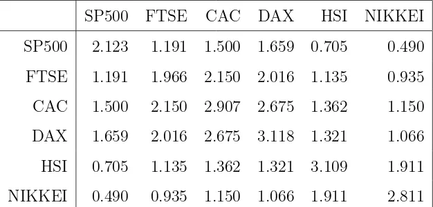
no safe assets. The covariance matrix of returns suggests stronger positive

correlations among western countries. The correlations between western and

oriental markets are less prominent, which carries significance for global

di-versifications.

As is seen in Table 1, daily returns of stock indexes exhibit substantial

skewness for most markets. The Lilliefors tests (Kolmogorov-Smirnov test

with estimated parameters) and Jarque-Bera test provides strong evidence

against normality with p value smaller than 0.001.

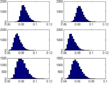
The departure from normality can also be seen from the Bayesian residual

test. We first fit the MSGM model with one regime and one state, which

is effectively a model of multivariate normal returns. We conduct a series

of residual tests by normalizing the historical returns using the posterior

draws of the mean and covariance matrix. If the returns are indeed normally

distributed, then the classical Kolmogorov-Smirnov test should accept the

null. The histogram of the test statistics are reported in Figure 1. The six

panels correspond to the six assets in sequence. Since we have a fairly large

sample size of more than 2000 observations, the 1% significance critical value

of the test statistics can be approximated by 1.63/√T, which is about 0.03.

Figure 1 shows that test statistics are larger than the critical value in every

circumstance so that the normality can be decisively rejected.

We also go through the above tests for subsamples of the data set.

did not report the results in the text. Noted that all the normality tests

are conducted on the basis of individual asset returns. Once the normality

is rejected at individual level, the joint normality is automatically rejected

(The reverse is not true). We therefore conclude that it is necessary to adopt

more flexible distributions to model asset returns.

In this application, we fit the MSGM model with three Markov switching

regimes, each with three states in the Gaussian mixture. The covariance

matrix is assumed to be invariant across regimes and states. The posterior

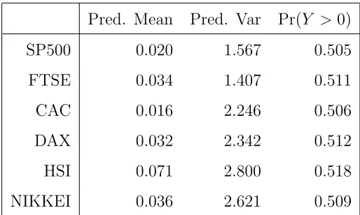
predictive distributions of asset returns are reported in Table 3. The

pre-dicted mean returns are positive, in contrast to the slightly negative mean

returns over the entire sample. The positive returns prediction might due to

the fact that at the end of our sample period, the return series tend to be

positive and thus in a high-return regime. The variances of the predictive

distributions contain triple uncertainties, namely the uncertainty over the

regimes and states, the uncertainty over the parameters and the uncertainty

over the future disturbances. However, Table 3 shows that for each asset

the predictive variance is smaller than the sample variance (which effectively

corresponds to a model with one regime and one state). That implies the

MSGM model better captures the non-normality feature of the data and

improves precision of the prediction.

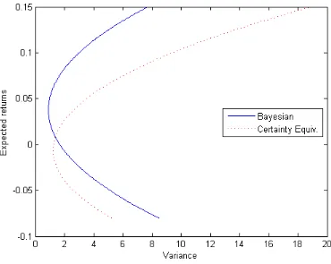
Using the draws from the posterior predictive distribution, Figure 2 plots

the Bayesian mean-variance frontier. For comparison, we also provide the

mean-variance frontier with certainty equivalent approach. The two curves

present different mean-variance trade-offs. For a given variance, the Bayesian

Mean-variance frontier may not be directly relevant to decision making

in the presence of non-normality. The next step is to estimate the optimal

portfolio weights which maximize the expected utility. We use a Tylor

ap-proximation up to the fourth order and assume that the portfolio manager

has a CARA utility. Table 4 shows the optimal weights with risk aversion

coefficients 1, 3, 5, 7, 9 and 11. The optimal weight on the third and fourth

assets are negative, which requires short selling. Table 5 provides optimal

weights when short selling is not allowed.

6. Conclusion

Departure from normality and parameter estimation risk are two major

barriers to the implementation of the Markowitz portfolio selection. This

pa-per attempts to addresses the two issues in a unified Bayesian framework, in

which deviation from normality is captured by a Markov switching Gaussian

mixture distribution and parameter uncertainty is reflected in the posterior

predictive distribution of asset returns. We develop a Gibbs sampling

proce-dure to obtain draws from the posterior distribution as well as draws from the

predictive density. Then the portfolio weights can be optimally constructed

so as to maximize the expected utility of investors.

To illustrate our approach, we considered a simplified version of global

di-versification of investing in several leading stock market indexes. The

descrip-tive statistics provide strong evidence against normality of high frequency

index returns. A model with four regimes and four states is used to predict

the future returns, and the associated optimal portfolios are also reasonably

Ane, T., Geman, H., 2000. Order flow, transaction clock, and normality of

asset returns. Journal of Finance 55 (5), 2259–2284.

Baum, L. E., Eagon, J. A., 1967. An inequality with applications to statistical

estimation for probabilistic functions of markov processes and to a model

for ecology. Bulletin of American Mathematical Society 73, 360–363.

Baum, L. E., Petrie, T., 1966. Statistical inference for probabilistic functions

of finite state markov chains. The Annals of Mathematical Statistics 37 (6),

1554–1563.

Baum, L. E., Petrie, T., Soules, G., Weiss, N., 1970. A maximization

tech-nique occurring in the statistical analysis of probabilistic functions of

markov chains. The Annals of Mathematical Statistics 41 (1), 164–171.

Black, F., Litterman, R., 1992. Global portfolio optimization. Financial

An-alysts Journal 48, 28C43.

Blattberg, R. C., Gonedes, N. J., 1974. A comparison of the stable and

student distributions as statistical models for stock prices. The Journal of

Business 47 (2), 244–80.

Buckley, I., Saunders, D., Seco, L., 2008. Portfolio optimization when

as-set returns have the gaussian mixture distribution. European Journal of

Operational Research 185 (3), 1434–1461.

Calvet, L. E., Fisher, A. J., 2004. How to forecast long-run volatility: Regime

switching and the estimation of multifractal processes. Journal of Financial

Celeux, G., Hurn, M., Robert, C. P., 2000. Computational and inferential

difficulties with mixture posterior distributions. Journal of the American

Statistical Association 95 (451), 957–970.

Chib, S., 1996. Calculating posterior distributions and modal estimates in

markov mixture models. Journal of Econometrics 75 (1), 79–97.

Chopra, V. K., Ziemba, W. T., 1993. The effect of errors in means,

vari-ances, and covariances on optimal portfolio choice. Journal of Portfolio

Management 19, 6–11.

Dickinson, J. P., 1974. The reliability of estimation procedures in portfolio

analysis. Journal of Financial and Quantitative Analysis 9 (03), 447–462.

Fama, E. F., 1965. The behavior of stock-market prices. The Journal of

Business 38 (1), pp. 34–105.

Fruhwirth-Schnatter, S., 2001. Markov chain monte carlo estimation of

clas-sical and dynamic switching and mixture models. Journal of the American

Statistical Association 96 (453), 194–209.

Geweke, J., 2007. Interpretation and inference in mixture models: Simple

mcmc works. Computational Statistics and Data Analysis 51 (7), 3529–

3550.

Hamilton, J., 2005. Regime-switching models.

dss.ucsd.edu/ jhamilto/palgrav1.pdf.

Hamilton, J. D., 1989. A new approach to the economic analysis of

Harvey, C., Liechty, J., Liechty, M., Muller, P., 2010. Portfolio selection with

higher moments. Quantitative Finance 10 (5), 469–485.

Harvey, C. R., Siddique, A., 2000. Conditional skewness in asset pricing tests.

Journal of Finance 55 (3), 1263–1295.

Jasra, A., Holmes, C. C., Stephens, D. A., 2005. Markov chain monte carlo

methods and the label switching problem in bayesian mixture modeling.

Statistical Science 20 (1), 50–67.

Jobson, J. D., Korkie, B., 1980. Estimation for markowitz efficient portfolios.

Journal of the American Statistical Association 75 (371), 544–554.

Jondeau, E., Rockinger, M., 2006. Optimal portfolio allocation under higher

moments. European Financial Management 12 (1), 29–55.

Kim, C.-J., Piger, J., Startz, R., 2008. Estimation of markov

regime-switching regression models with endogenous regime-switching. Journal of

Econo-metrics 143 (2), 263–273.

Kraus, A., Litzenberger, R. H., 1976. Skewness preference and the valuation

of risk assets. Journal of Finance 31 (4), 1085–1100.

Krolzig, H.-M., 1997. Markov-switching vector autoregressions : modelling,

statistical inference, and application to business cycle analysis. Springer.

Lucas, R. E., 1978. Asset prices in an exchange economy. Econometrica

46 (6), 1429–1445.

Michaud, R. O., Michaud, R. O., 2008. Efficient asset management: A

prac-tical guide to stock portfolio optimization and asset allocation.

Peiro, A., 1999. Skewness in financial returns. Journal of Banking and

Fi-nance 23 (6), 847 – 862.

Rabiner, L. R., 1989. A tutorial on hidden markov models and selected

appli-cations in speech recognition. In: Proceedings of the IEEE. pp. 257–286.

Roman, D., Mitra, G., Spagnolo, N., 2010. Hidden markov models for

fi-nancial optimization problems. IMA Journal of Management Mathematics

21 (2), 111–129.

Scherer, B., 2002. Portfolio resampling: Review and critique. Financial

An-alysts Journal 58 (6), 98–109.

Sims, C. A., Zha, T., 2006. Were there regime switches in u.s. monetary

policy? American Economic Review 96 (1), 54–81.

Turner, C. M., Startz, R., Nelson, C. R., 1989. A markov model of

het-eroskedasticity, risk, and learning in the stock market. Journal of Financial

SP500 FTSE CAC DAX HSI NIKKEI

Mean -0.005 -0.008 -0.024 -0.005 0.003 -0.031

Skewness -0.193 0.013 0.117 0.010 -0.216 -0.408

Kurtosis 9.180 9.818 8.667 8.585 12.586 9.528

Lilliefors 0.080 0.079 0.071 0.068 0.080 0.058

p-val 0.001 0.001 0.001 0.001 0.001 0.001

Jarque-Bera 4258.0 5162.4 3572.5 3463.4 10225.5 4806.2

p-val 0.001 0.001 0.001 0.001 0.001 0.001

Table 1: Descriptive statistics of daily percentage asset returns

SP500 FTSE CAC DAX HSI NIKKEI

SP500 2.123 1.191 1.500 1.659 0.705 0.490

FTSE 1.191 1.966 2.150 2.016 1.135 0.935

CAC 1.500 2.150 2.907 2.675 1.362 1.150

DAX 1.659 2.016 2.675 3.118 1.321 1.066

HSI 0.705 1.135 1.362 1.321 3.109 1.911

NIKKEI 0.490 0.935 1.150 1.066 1.911 2.811

Pred. Mean Pred. Var Pr(Y >0)

SP500 0.020 1.567 0.505

FTSE 0.034 1.407 0.511

CAC 0.016 2.246 0.506

DAX 0.032 2.342 0.512

HSI 0.071 2.800 0.518

NIKKEI 0.036 2.621 0.509

Table 3: Summary of the posterior predictive asset returns with a three-regime, three-state

MSGM model

1 3 5 7 9 11

SP500 40.5 39.5 38.3 37.1 35.9 34.7

FTSE 83.3 87.8 90.2 92.4 94.7 97.0

CAC -33.5 -30.0 -31.5 -33.5 -35.5 -37.7

DAX -17.0 -22.5 -22.4 -21.9 -21.3 -20.6

HSI 6.9 1.2 0.8 1.3 2.0 2.9

NIKKEI 19.7 24.1 24.7 24.6 24.2 23.8

Table 4: Optimal portfolio weights (in percentage) under different risk aversion coefficients

while short selling is allowed. The expected utility is approximated by the Taylor expansion

1 3 5 7 9 11

SP500 33.4 29.3 26.6 26.3 25.6 24.5

FTSE 44.9 52.7 54.8 55.7 56.2 55.9

CAC 0.0 0.0 0.0 0.0 0.0 0.0

DAX 0.0 0.0 0.9 0.0 0.1 1.1

HSI 4.6 2.2 0.6 0.2 0.0 1.2

NIKKEI 17.1 15.8 17.1 17.8 18.2 17.3

Table 5: Optimal portfolio weights (in percentage) under different risk aversion coefficients

while short selling is not allowed. The expected utility is approximated by the Taylor

Figure 1: Bayesian residual Kolmogorov-Smirnov test statistics. The six panels correspond

to SP500, FTSE, CAC, DAX, HSI, NIKKEI respectively. Under the null of normality, the

Figure 2: A comparison of the classic mean variance frontier (certainty equivalence

solu-tion) with the mean variance frontier using the posterior predictive distribution of asset