Mathematics Dissertations Department of Mathematics and Statistics
12-14-2017
Bayesian Methods in Brain Connectivity Change
Point Detection with EEG Data and Genetic
Algorithm
Bing Liu
Follow this and additional works at:https://scholarworks.gsu.edu/math_diss
This Dissertation is brought to you for free and open access by the Department of Mathematics and Statistics at ScholarWorks @ Georgia State University. It has been accepted for inclusion in Mathematics Dissertations by an authorized administrator of ScholarWorks @ Georgia State University. For more information, please [email protected].
Recommended Citation
Liu, Bing, "Bayesian Methods in Brain Connectivity Change Point Detection with EEG Data and Genetic Algorithm." Dissertation, Georgia State University, 2017.
BING LIU
Under the Direction of Jing Zhang, PhD
ABSTRACT
Human brain is processing a great amount of information everyday, and our brain
regions are organized optimally for this information processing. There have been increasing
number of studies focusing on functional or effective connectivity in human brain regions
in the last decade. In this dissertation, Bayesian methods in Brain connectivity change
point detection are discussed. First, a review of state-of-the-art Bayesian-inference-based
methods applied to functional magnetic resonance imaging (fMRI) data is carried out, three
methods are reviewed and compared. Second, the Bayesian connectivity change point model
is extended to change point analysis in electroencephalogram (EEG) data, and the ability
of EEG measures of frontal and temporo-parietal activity during mindfulness therapy to
is proposed and proved to be more efficient in change point detection. And due to the good
parallel performance of GA, the change point detection method can be parallelized in GPU
or multi-processor computers as a future work. Furthermore, a more advanced Bayesian
bi-cluster connectivity change point model is developed to simultaneously detect change
point of each subject within a group, and cluster subjects into different groups according to
their change point distribution and connectivity dynamics. The method is also validated on
experimental datasets. After discussing brain change point detection, a review of Bayesian
analysis of complex mutations in HBV HCV and HIV studies is also included as part of my
Ph.D. work. Finally, conclusions are drawn and future work is discussed.
INDEX WORDS: Bayesian inference, Brain network, Change point, Connectivity
by
BING LIU
A Dissertation Submitted in Partial Fulfillment of the Requirements for the Degree of
Doctor of Philosophy
in the College of Arts and Sciences
Georgia State University
BING LIU
Committee Chair: Jing Zhang
Committee: Yi Pan
Xin Qi
Ruiyan Luo
Electronic Version Approved:
Office of Graduate Studies
College of Arts and Sciences
Georgia State University
DEDICATION
suggestions and guidance while I was doing this dissertation research. Her insights and
knowledge always inspired me and I truly learned a lot from her. I’d like to give my special
thanks to Dr. Yi Pan for sharing his valuable knowledge and all the help in our collaboration.
My special thanks to Dr. Xin Qi and Dr. Ruiyan Luo, for reviewing my dissertation and
providing helpful advices.
Special thanks to Dr. Jessica Turner and Dr. Matthew Turner for their generous help
in our EEG study and providing the EEG data for my dissertation research.
Special thanks to Dr. Xuan Guo, Dr. Xiuchun Xiao, Xueli Xiao, and Le Chen for their
valuable contributions in our collaboration.
My gratitude also goes to our Chair Dr. Guantao Chen, who offered me advice and
help. To Dr. Gengsheng Qin, who is always patient and gives me courage. To Dr. Yichuan
Zhao, who organized wonderful statistics colloquium which provide us the opportunities to
connect academia and industry. And to my undergraduate advisor, Dr. Danhui Yi, who led
me into the field of statistics and gave me opportunities to practice while learning.
Special thanks to all the faculty, staff and students in the Department of Mathematics
and Statistics at Georgia State University.
Special thanks to Brain and Behavior Seed Grant from Georgia State University.
Furthermore, I would like to thank my all friends who helped me when I faced difficulties.
Last but not least, I want to thank my dear parents Jingdong Liu and Yufang Liu, my
girlfriend Yuyin Shi and my relatives who always support me once I make my decision to do
something. I cannot achieve anything without your unconditional support. I love you all!
TABLE OF CONTENTS
ACKNOWLEDGEMENTS . . . v
LIST OF TABLES . . . x
LIST OF FIGURES . . . xi
LIST OF ABBREVIATIONS . . . xxi
CHAPTER 1 INTRODUCTION . . . 1
1.1 Brain Connectivity . . . 1
1.2 Brain Connectivity Change Points Detection and Dynamics Explo-ration . . . 2
1.3 Main Contributions . . . 3
1.4 Structure of the Rest of the Dissertation . . . 5
CHAPTER 2 A REVIEW OF BAYESIAN INFERENCE FOR FUNC-TIONAL DYNAMICS EXPLORING IN FMRI DATA . 6 2.1 Bayesian Inference . . . 6
2.2 Bayesian Magnitude Change Point Model . . . 9
2.3 Bayesian Functional Connectivity Change Point Model . . . 11
2.4 Bayesian Change Point Model Using One-Level MCMC Scheme 12 2.5 Dynamic Bayesian Variable Partition Model . . . 13
2.5.1 Chain-Dependence Model . . . 14
2.5.2 V-Dependence Model . . . 14
2.5.3 Dynamic Bayesian Variable Partition Model . . . 15
2.6 DBVPM Using Two-Level MCMC Scheme . . . 16
3.3.1 Data Acquisition Device . . . 21
3.3.2 Data Preprocessing . . . 23
3.4 Experimental Results . . . 23
3.4.1 Experimental Design . . . 24
3.4.2 Results . . . 26
3.5 Results on EEG Data from Mindfulness Therapy for Dysfunctional Anxiety Patients . . . 47
3.5.1 Recorded Data Description . . . 47
3.5.2 Results . . . 48
3.6 Summary . . . 50
CHAPTER 4 AN OPTIMIZED BAYESIAN FUNCTIONAL CONNEC-TIVITY CHANGE POINT MODEL WITH GENETIC AL-GORITHM . . . 51
4.1 Introduction . . . 51
4.2 Modified Genetic Algorithm and Bayesian Inference Theory . . 53
4.2.1 Modified Genetic Algorithm . . . 53
4.2.2 Bayesian Connectivity Change Poing Model . . . 57
4.3 Simulation Study and Real Data Application . . . 58
4.3.1 Simulation Study I . . . 58
4.3.2 Simulation Study II . . . 62
4.3.3 Real Data Application . . . 67
CHAPTER 5 BAYESIAN BI-CLUSTER CONNECTIVITY CHANGE POINT
MODEL . . . 71
5.1 Introduction . . . 71
5.2 Methodology . . . 72
5.2.1 Bayesian Bi-cluster Connectivity Change Point Model . . . 72
5.2.2 Two-level MCMC Scheme . . . 77
5.3 Experimental Results . . . 78
5.4 Conclusion and Future Work . . . 82
CHAPTER 6 OTHER TOPICS: BAYESIAN ANALYSIS OF COMPLEX MUTATIONS IN HBV HCV AND HIV STUDIES . . 83
6.1 Introduction . . . 83
6.2 Bayesian Methods in HBV, HCV and HIV Studies . . . 86
6.2.1 Bayesian Variable Partition Model . . . 87
6.2.2 Bayesian Partition on Dual Usage of Co-receptor Model . . . 90
6.2.3 Metropolis-Hastings Algorithm . . . 91
6.2.4 Recursive Model Selection . . . 92
6.3 Applications of Bayesian Methodology to HBV, HCV and HIV s-tudies . . . 94
6.3.1 Applications in HBV studies . . . 94
6.3.2 Applications in HCV studies . . . 94
6.3.3 Applications in HIV studies . . . 98
6.4 Summary and Discussion . . . 99
CHAPTER 7 CONCLUSIONS AND FUTURE WORK . . . 100
REFERENCES . . . 103
LIST OF TABLES
Table 3.1 Experiment 1 (in seconds) . . . 24
Table 3.2 Experiment 2 (in minutes) . . . 24
Table 3.3 Experiment 3 (in seconds) . . . 25
Table 3.4 Experiment 4 (in minutes) . . . 25
Table 3.5 List of paired subjects . . . 47
Table 3.6 Poisson rates of test subjects in different sessions (p=-2000). . . . 49
Table 4.1 Comparison of computational cost (time in ms) . . . 62
Table 4.2 Comparison of computational cost (time in ms) . . . 67
Table 4.3 Results on real data application . . . 68
Table 6.1 A summary of results from applications of Bayesian methods to HBV studies . . . 95
Table 6.2 Single positions result summary . . . 95
Table 6.3 Dependence structure inferred by RMS in detail . . . 97
time point i. . . 8
Figure 2.2 An ROI signal with one magnitude change point at time point T100. 9
Figure 2.3 Three ROI signals with one connectivity change point at time point
T100. The multivariate normal distribution inside the block T1-T100 of
color blue is different from the distribution of signal in the rest block
of color orange. . . 12
Figure 2.4 Three ROIs signals with one temporal change point at time pointT100.
Left block shows a chain dependence structure with signalsi→j →k
and the right block shows a V-dependence structure with signals i→
j ←k. . . 14
Figure 3.1 EPOC/EPOC+ headset device with 14 electrodes. Image from
EMO-TIV EPOC User Manual. . . 21
Figure 3.2 EPOC/EPOC+ headset placement demonstration. Image from
EMO-TIV EPOC User Manual. . . 22
Figure 3.3 Experiment 1: Traceplot shows the convergence of MCMC chains
(p=0). . . 27
Figure 3.4 Experiment 1: Change points detected by BCCPM for five repeated
MCMC chains (p=0). Red dotted lines are the locations of designed
Figure 3.5 Experiment 1: Change points detected by BCCPM for the best
de-tection result (p=0). Red dotted lines are the locations of designed
change points. . . 28
Figure 3.6 Experiment 1: Traceplot shows the convergence of MCMC chains
(p=-1000). . . 28
Figure 3.7 Experiment 1: Change points detected by BCCPM for five
repeat-ed MCMC chains (p=-1000). Rrepeat-ed dottrepeat-ed lines are the locations of
designed change points. . . 29
Figure 3.8 Experiment 1: Change points detected by BCCPM for the best
detec-tion result (p=-1000). Red dotted lines are the locadetec-tions of designed
change points. . . 29
Figure 3.9 Experiment 1: Traceplot shows the convergence of MCMC chains
(p=-2000). . . 30
Figure 3.10 Experiment 1: Change points detected by BCCPM for five
repeat-ed MCMC chains (p=-2000). Rrepeat-ed dottrepeat-ed lines are the locations of
designed change points. . . 30
Figure 3.11 Experiment 1: Change points detected by BCCPM for the best
detec-tion result (p=-2000). Red dotted lines are the locadetec-tions of designed
change points. . . 31
Figure 3.12 Experiment 1: Change points detected by BCCPM for the best
detec-tion result (p=-4000). Red dotted lines are the locadetec-tions of designed
change points. . . 31
Figure 3.13 Experiment 1: Change points detected by BCCPM for the best
detec-tion result (p=-6000). Red dotted lines are the locadetec-tions of designed
change points. . . 32
Figure 3.16 Experiment 2: Change points detected by BCCPM for the best
de-tection result (p=0). Red dotted lines are the locations of designed
change points. . . 33
Figure 3.17 Experiment 2: Traceplot shows the convergence of MCMC chains
(p=-1000). . . 33
Figure 3.18 Experiment 2: Change points detected by BCCPM for five
repeat-ed MCMC chains (p=-1000). Rrepeat-ed dottrepeat-ed lines are the locations of
designed change points. . . 34
Figure 3.19 Experiment 2: Change points detected by BCCPM for the best
detec-tion result (p=-1000). Red dotted lines are the locadetec-tions of designed
change points. . . 34
Figure 3.20 Experiment 2: Traceplot shows the convergence of MCMC chains
(p=-2000). . . 35
Figure 3.21 Experiment 2: Change points detected by BCCPM for five
repeat-ed MCMC chains (p=-2000). Rrepeat-ed dottrepeat-ed lines are the locations of
designed change points. . . 35
Figure 3.22 Experiment 2: Change points detected by BCCPM for the best
detec-tion result (p=-2000). Red dotted lines are the locadetec-tions of designed
Figure 3.23 Experiment 2: Change points detected by BCCPM for the best
detec-tion result (p=-4000). Red dotted lines are the locadetec-tions of designed
change points. . . 36
Figure 3.24 Experiment 2: Change points detected by BCCPM for the best
detec-tion result (p=-6000). Red dotted lines are the locadetec-tions of designed
change points. . . 36
Figure 3.25 Experiment 3: Traceplot shows the convergence of MCMC chains
(p=0). . . 37
Figure 3.26 Experiment 3: Change points detected by BCCPM for five repeated
MCMC chains (p=0). Red dotted lines are the locations of designed
change points. . . 37
Figure 3.27 Experiment 3: Change points detected by BCCPM for the best
de-tection result (p=0). Red dotted lines are the locations of designed
change points. . . 38
Figure 3.28 Experiment 3: Traceplot shows the convergence of MCMC chains
(p=-1000). . . 38
Figure 3.29 Experiment 3: Change points detected by BCCPM for five
repeat-ed MCMC chains (p=-1000). Rrepeat-ed dottrepeat-ed lines are the locations of
designed change points. . . 39
Figure 3.30 Experiment 3: Change points detected by BCCPM for the best
detec-tion result (p=-1000). Red dotted lines are the locadetec-tions of designed
change points. . . 39
Figure 3.31 Experiment 3: Traceplot shows the convergence of MCMC chains
tion result (p=-2000). Red dotted lines are the locations of designed
change points. . . 41
Figure 3.34 Experiment 3: Change points detected by BCCPM for the best
detec-tion result (p=-4000). Red dotted lines are the locadetec-tions of designed
change points. . . 41
Figure 3.35 Experiment 3: Change points detected by BCCPM for the best
detec-tion result (p=-6000). Red dotted lines are the locadetec-tions of designed
change points. . . 41
Figure 3.36 Experiment 4: Traceplot shows the convergence of MCMC chains
(p=0). . . 42
Figure 3.37 Experiment 4: Change points detected by BCCPM for five repeated
MCMC chains (p=0). Red dotted lines are the locations of designed
change points. . . 42
Figure 3.38 Experiment 4: Change points detected by BCCPM for the best
de-tection result (p=0). Red dotted lines are the locations of designed
change points. . . 43
Figure 3.39 Experiment 4: Traceplot shows the convergence of MCMC chains
(p=-1000). . . 43
Figure 3.40 Experiment 4: Change points detected by BCCPM for five
repeat-ed MCMC chains (p=-1000). Rrepeat-ed dottrepeat-ed lines are the locations of
Figure 3.41 Experiment 4: Change points detected by BCCPM for the best
detec-tion result (p=-1000). Red dotted lines are the locadetec-tions of designed
change points. . . 44
Figure 3.42 Experiment 4: Traceplot shows the convergence of MCMC chains
(p=-2000). . . 45
Figure 3.43 Experiment 4: Change points detected by BCCPM for five
repeat-ed MCMC chains (p=-2000). Rrepeat-ed dottrepeat-ed lines are the locations of
designed change points. . . 45
Figure 3.44 Experiment 4: Change points detected by BCCPM for the best
detec-tion result (p=-2000). Red dotted lines are the locadetec-tions of designed
change points. . . 46
Figure 3.45 Experiment 4: Change points detected by BCCPM for the best
detec-tion result (p=-4000). Red dotted lines are the locadetec-tions of designed
change points. . . 46
Figure 3.46 Experiment 4: Change points detected by BCCPM for the best
detec-tion result (p=-6000). Red dotted lines are the locadetec-tions of designed
change points. . . 46
Figure 3.47 Comparison of number of change points of Subject 1 from therapy
session 1 to 4 to 7. The number of change points decreases as sessions
go on (p=-2000). . . 48
Figure 3.48 In session 7, Subject 1 and Subject 5 have different change point
pat-terns (p=-2000). . . 50
Figure 4.4 Convergence curve for network (a)-(f) (Left column is results of
MCMC-Based-BCCPM. Right column is results of GA-Based-BCCPM). 60
Figure 4.5 Change point detection results for network (a)-(f) (Left column is
re-sults of MCMC-Based-BCCPM. Right column is rere-sults of
GA-Based-BCCPM). . . 61
Figure 4.6 Eight different structures of dynamic networks and their change-point
distributions. . . 63
Figure 4.7 Convergence curves for networks (a)-(h) (Left column shows results
from MCMC-Based-BCCPM. Right column shows results from
GA-Based-BCCPM). . . 65
Figure 4.8 Change point detection results for network (a)-(h) (Left column shows
results from MCMC-Based-BCCPM. Right column shows results from
GA-Based-BCCPM). . . 66
Figure 4.9 Top: Detected change point shown in blue ridges with designed blocks
split by red dotted lines of subject 6. Bottom: Functional interaction
patterns searched by PC algorithm from three temporal blocks: I. face,
II. shape, III. fixation. . . 69
Figure 5.1 Data matrix ofY and block indicator vector I, whereyt are the values
of all ROIs at time t(thet-th column in the matrix),Yj are the values
of the j-th ROI at all times (the j-th row in the matrix) and It is a
Figure 5.2 Three subjects in two clustering groups. . . 76
Figure 5.3 Work flow of the two-level MCMC scheme. . . 78
Figure 5.4 Experimental design: Five subjects with two group clusterings and
their change point distributions. . . 79
Figure 5.5 Overall convergence curve. . . 79
Figure 5.6 Convergence curve for lower level MCMC in Group 1 (Subjects 1,2). 80
Figure 5.7 Change point detection result for Group 1 (Subjects 1,2). . . 80
Figure 5.8 Convergence curve for lower level MCMC in Group 2 (Subjects 3,4,5). 81
Figure 5.9 Change point detection result for Group 2 (Subjects 3,4,5). . . 81
Figure 6.1 The chain-dependence model structure. Colors indicate different sets
of variables. . . 93
Figure 6.2 The V-dependence model structure. Colors indicate different sets of
variables. Notice that variables in U are marginally independent of
the variables in W. . . 93
Figure 6.3 Flowchart of detected mutation positions and position combinations in
the pretreatment sequence of patients who respond to the treatment. 96
Figure 6.4 Flowchart of detected mutation positions and position combinations
in the pretreatment sequence of patients who don’t respond to the
treatment. . . 97
Figure A.1 Experiment 1: Traceplot shows the convergence of MCMC chains
6000). . . 116
Figure A.4 Experiment 1: Change points detected by BCCPM for five
repeat-ed MCMC chains (p=-6000). Rrepeat-ed dottrepeat-ed lines are the locations of
designed change points. . . 116
Figure A.5 Experiment 2: Traceplot shows the convergence of MCMC chains
(p=-4000). . . 117
Figure A.6 Experiment 2: Change points detected by BCCPM for five
repeat-ed MCMC chains (p=-4000). Rrepeat-ed dottrepeat-ed lines are the locations of
designed change points. . . 117
Figure A.7 Experiment 2: Traceplot shows the convergence of MCMC chains
(p=-6000). . . 118
Figure A.8 Experiment 2: Change points detected by BCCPM for five
repeat-ed MCMC chains (p=-6000). Rrepeat-ed dottrepeat-ed lines are the locations of
designed change points. . . 118
Figure A.9 Experiment 3: Traceplot shows the convergence of MCMC chains
(p=-4000). . . 119
Figure A.10 Experiment 3: Change points detected by BCCPM for five
repeat-ed MCMC chains (p=-4000). Rrepeat-ed dottrepeat-ed lines are the locations of
Figure A.11 Experiment 3: Traceplot shows the convergence of MCMC chains
(p=-6000). . . 120
Figure A.12 Experiment 3: Change points detected by BCCPM for five
repeat-ed MCMC chains (p=-6000). Rrepeat-ed dottrepeat-ed lines are the locations of
designed change points. . . 120
Figure A.13 Experiment 4: Traceplot shows the convergence of MCMC chains
(p=-4000). . . 121
Figure A.14 Experiment 4: Change points detected by BCCPM for five
repeat-ed MCMC chains (p=-4000). Rrepeat-ed dottrepeat-ed lines are the locations of
designed change points. . . 121
Figure A.15 Experiment 4: Traceplot shows the convergence of MCMC chains
(p=-6000). . . 122
Figure A.16 Experiment 4: Change points detected by BCCPM for five
repeat-ed MCMC chains (p=-6000). Rrepeat-ed dottrepeat-ed lines are the locations of
designed change points. . . 122
• BMCPM - Bayesian Magnitude Change Point Model
• BVP - Bayesian Variable Partition
• CI - Confidence Interval
• DBVPM - Dynamic Bayesian Variable Partition Model
• EEG - Electroencephalography
• fMRI - Functional magnetic resonance imaging
• GA - Genetic algorithm
• GSU - Georgia State University
• HBV - Hepatitis B virus
• HCV - Hepatitis C virus
• HIV - human immunodeficiency virus
• i.i.d. - independent identically distributed
• MCMC - Markov chain Monte Carlo
• M-H - Metropolis-Hastings
• PTSD - Post-traumatic Stress Disorder
• RMS - Recursive Model Selection
CHAPTER 1
INTRODUCTION
1.1 Brain Connectivity
Our brain processes a large number of information everyday, and most of the
infor-mation is processed by different but related brain regions. The paradigm in neuroscience
is that the anatomical and functional connections between our brain regions are organized
optimally for information processing [39]. Brain connectivity often refers to three
pattern-s of linkpattern-s, dependenciepattern-s or interactionpattern-s: anatomical connectivity, functional connectivity,
effective connectivity [79].
• Anatomical connectivity, also notes as anatomical links or structure connectivity, which
is in a form of a network of structural connections linking neurons or elements of
neu-ronal systems. At shorter time scales (seconds to minutes), the anatomical connections
are relatively stable, while at longer time scales (hours to days), it is likely to observe
some plasticity.
• Functional connectivity, often called statistical dependencies, on the other hand, is
based on statistical concepts. It captures the dependency between distributed and
remote neuronal units. Theses statistical dependencies may be inferred by estimating
the correlation or covariance, spectral coherence or phase-locking, and they are highly
time dependent.
• Effective connectivity, also called causal interactions, describes the effect from one
neural on another directionally. It can be considered as a combination of structural
and functional connectivities. Oftentimes, these casual effects can be analyzed by time
dependent (BOLD) signal [39].
1.2 Brain Connectivity Change Points Detection and Dynamics Exploration
Recently in the research area of functional magnetic resonance imaging (fMRI), an
in-creasing interest comes in the dynamic connectivity of brain regions which communicate
one from another. Lindquist et al. [48] proposed a statistical method, named as
Hierarchi-cal Exponentially Weighted Moving Average (HEWMA), on fMRI data to detect the state
change of BOLD signals in response to stimulus. Cribben et al. [12] developed a Dynamic
Connectivity Regression method, which is a data-driven method for detecting functional
con-nectivity change points. Independent component analysis (ICA) method, including dynamic
spatial ICA, was developed by Sako¨glu et al. [75] to investigate the connectivity dynamics.
Also, sliding-time-window-based approaches were designed to capture the dynamics of brain
functional interactions across different time windows [41][103][67][53][102][1]. For example,
Allen et al. [1] described an approach to assess whole-brain functional connectivity (FC)
dynamics based on spatial ICA, sliding-time-window correlation analysis, and k-means
clus-tering of windowed correlation matrices, and it revealed unanticipated FC states which were
strongly different from stationary connectivity patterns. Li et al. [41] derived functional
connectomes (FCs) to characterize brain conditions from resting-state fMRI data and then
FCs were divided into quasi-stable segments temporally via a sliding-time-window approach.
In [103], a novel framework was designed by the combination of sliding-window approach and
multiview spectral clustering to extract temporally dynamic functional connectome patterns
for resting-state networks, and the four detected clusters are believed to play critical roles in
on hidden Markov models was presented to cluster and label the brains functional states,
represented by a large-scale functional connectivity matrix and derived via an overlapping
sliding-time-window approach. The framework achieved decent classification performance
on the data including 25 ADHD (attention-deficit/hyperactivity disorder) patients and 49
normal controls. Lv et al. [53] also adopted the sliding-window-based method and
em-ployed a dynamic programming strategy to infer functional information transition routines
on structural networks and identified the hub routers that participate in these routines most
frequently.
Inspired by the multivariate graphical models based on Bayesian networks, which has
been shown to be robust and reliable in estimating functional interactions and less sensitive to
noise in the fMRI signals [73][81][77], recently, several Bayesian-inference-based methods were
proposed to infer global functional interactions within brain networks and their temporal
transition boundaries [46][43][101][64][65][45]. By evaluating and estimating both simulated
and real data, Bayesian-inference-based methods are proved to be more powerful approaches
for analysis fMRI data comparing to the methods mentioned above.
1.3 Main Contributions
In this dissertation, the main contributions are summarized as follows:
• A review of state-of-the-art Bayesian-inference-based methods applied to functional
magnetic resonance imaging (fMRI) data:
– Bayesian Magnitude Change Point Model;
– Bayesian Functional Connectivity Change Point Model;
– Dynamic Bayesian Variable Partition Model;
• An extension of Bayesian connectivity change point model to EEG data change point
analysis:
• An optimized method for Bayesian connectivity change point model with genetic
al-gorithm:
– combine Bayesian connectivity change point model with a modified genetic
algo-rithm;
– optimize the evolutionary procedure to improve the detection accuracy;
– decrease the time consumption/computational cost;
– validate the optimized method on simulated and real data.
• A Bayesian bi-cluster connectivity change point model:
– detect change point of each subject within a group, and simultaneously
– cluster subjects into different groups according to their change point distribution
with bayesian framework;
– develop a two level MCMC scheme to sample from the posterior distribution;
– validate the proposed method on experimental datasets;.
• Other topics: a review of Bayesian analysis of complex mutations in HBV HCV and
HIV studies:
– review the Bayesian-inference-based methods applied to Hepatitis B virus (HBV),
Hepatitis C virus (HCV) and the human immunodeficiency virus (HIV) studies
with a focus on the detection of the viral mutations and various problems which
– summarize the Bayesian Variable Partition (BVP) model, and the Recursive
Mod-el SMod-election (RMS) procedure, which are designed to detect the mutations and to
further infer the detailed dependence structure among the interactions;
– summarize of the Bayesian methods applications toward these viruses studies,
where several important and useful results have been discovered;
1.4 Structure of the Rest of the Dissertation
The remainder of the dissertation focuses on the brain connectivity change point
detec-tion methods on both fMRI and EEG data. Chapter 2 reviews the current novel Bayesian
statistical inference methods for change point detection in fMRI data. Chapter 3 extends one
of the Bayesian change point detection methods from fMRI data to EEG data and focuses
on a preliminary research in testing the ability of EEG measures of frontal and
temporo-parietal activity during mindfulness therapy to track response to treatment, as an evaluation
of EEG as a physiological aid in therapy. Chapter 4 introduces an optimized method for
Bayesian Connectivity Change Point Model with genetic algorithm, which improves the
es-timate efficiency in detecting brain connectivity change points. Chapter 5 presents a more
advanced bi-cluster Bayesian inference model to simultaneously detect change points and
cluster subjects/patients according to their connectivity change point patterns, which
po-tentially can be used to classify healthy subjects and diseased patients. After discussing the
change point analysis, some other Bayesian methods applied in the fields of HBV, HCV and
HIV researches are also discussed and reviewed in Chapter 6 as part of this dissertation.
The material in Sections 2.1 through 2.7 of this chapter draws heavily on the author’s
previously published review article [31].
2.1 Bayesian Inference
Bayesian inference is a statistical inference method in which Bayes’ Rule is used to
update the estimated probability for a hypothesis as evidence is acquired, and it is a novel
method for combining prior knowledge with observed information to answer the questions
that researchers are usually interested in, like “what is the probability of getting lung cancer
for certain patients who does not smoke?”. It is a natural way to combine multiple
exper-iments information and fit realistic but complicated models. On the other hand, Bayesian
inference often has more computational cost and requires at least one of elicitation of
re-al subjective probability distributions of prior beliefs. The good thing is that sensitivity
analysis shows that the choice of prior does not strongly affect the inference.
Bayes’ Rule [90]
Ifθ is a discrete random variable with a probability mass function (p.m.f.), then
p(θ|y) = Pp(y|θ)p(θ)
ip(y|θi)p(θi))
(2.1)
When θ is continuous, Bayes’ Rule has the following form
p(θ|y) = p(θ, y) p(y) =
p(y|θ)p(θ) p(y) =
p(y|θ)p(θ)
R
ip(y|θ)p(θ))dθ
(2.2)
for a fixed y, and p(y|θ) is the likelihood. So Bayes’ Rule is considered as the posterior is
proportional to the product of prior and likelihood,
P osterior∝P rior×Likelihood
p(θ|y)∝p(θ)×p(y|θ)
(2.3)
Basics of the Bayesian Inference [90]
When we use Bayesian statistics to make inferences, consider
1. Setting up a probability model;
2. Applying the probability theory and the Bayes’ Rule.
For example, let (X1, ..., Xn) be an independent and identically distributed sample from
Binomial distribution Bin(n, π), where n is the sample size and π is the probability of
success. We have x|π ∼Bin(n, π). And the likelihood can be written as
p(x|π) =
n x
πx(1−π)n−x;π∈[0,1] (2.4)
If we want to make inference on π given x and n, a prior distribution p(π) for π is needed,
for example, we can choose a uniform distribution such that, π ∼U(0,1):
p(π) =
1, if 0≤π≤1
0, otherwise
(2.5)
Then by applying the Bayes’ Rule, we get
p(x, π) =
n x
πx(1−π)n−x
p(x) =
Z 1 0 n x
πx(1−π)n−xdπ = 1 n+ 1
p(π|x) = p(x, π)
x = (n+ 1)
n x
An fMRI data series consists of values at specific voxel of the image at some time point
t. These series are collected as aT-dimensional vector~y= (y1, y2, ..., yT). Suppose we record
the data based onm regions of interest (ROIs), then the dataset is an m×T matrixY. An
example can be found in Figure 2.1 [31].
Figure 2.1. Illustration of data matrixY with m ROIs and T time points, and a block
indicator vector I~, where yi is the values of all m ROIs at the time point i.
Our purpose is to use Bayesian analysis to make inference on the dynamic functional
connectivity change points. Define a block indicator I~= (I1, I2, ..., IT) to indicate the
loca-tions of change points in the m×T dataset. And this indicator becomes our parameter of
interest. Follow the Bayesian framework, we assume the prior of ~I is Bernoulli(0.5) so that
P(~I) =QT
the posterior distribution of p(I~|Y) can be obtained by
p(I~|Y)∼p(I~)p(Y|I~) (2.7)
Then a Markov chain Monte Carlo (MCMC) scheme can be used to sample the posterior
with a random initial block indicator.
Following these procedures, several models have been established and applied in change
point detection research. In the following sections in this chapter, three Bayesian models are
reviewed: Bayesian magnitude change point model, Bayesian connectivity change point
mod-el, and Bayesian variable partition model for detecting functional interaction and transition
patterns.
2.2 Bayesian Magnitude Change Point Model
Lian et al. proposed a Bayesian Magnitude Change Point Model (BMCPM) to detect
group-wise consistent magnitude change points [46]. A key feature of BMCPM is the
capa-bility to consider the group-wise fMRI signals of corresponding cortical landmarks across a
population of subjects and optimally determines the change boundaries. Magnitude change
points are defined as the temporal points dividing ROI data matrix into blocks which exhibit
substantial differences in brain states from each other. Figure 2.2 [31] demonstrates the basic
idea in BMCPM. One temporal change point located at time point T100 partitions the ROI
data matrix into two time blocks with different distributions.
Figure 2.2. An ROI signal with one magnitude change point at time pointT100.
Given a vector ~a = (a1, a2, ...at) i.i.d. from a normal distribution with mean µ and
Normal-p(a1, a2, ...at) = 1 2π r κ0 κt
Γ(νt/2) Γ(ν0/2)
(ν0σ02/2)ν0/2
(νtσt2/2)νt/2
(2.8)
Based on (2.8), given a data matrix A = (~a1, ~a2, ..., ~am), where~ai is a vector with the data
i.i.d. from the normal distribution as described before, and~ai’s are independent. Then, the
probability of A can be calculated as
p(A) = m
Y
i=1
p(~ai) (2.9)
where p(~ai) is computed as in (2.8)
To make inferences on the magnitude temporal change points, we define a block indicator
vector I~= (I1, I2, ..., IT), Ii = 1 if the ith observation is the beginning point of a block, and
Ii = 0 otherwise. Note that I1 = 1 as the first location is always being considered as a
change point. LetYi denote the data ofm ROIs at theith location. Then for data matrix Y
defined as in previous section, the likelihood given a block indicator vector can be calculated
as
p(Y|I~) =
P
Ij Y
i=1
p(Yi) (2.10)
where P(Yi) can be calculated using (2.9). Then the posterior of I~can be obtained by
p(I~|Y)∝p(I~)p(Y|I~) (2.11)
A Bernoulli distribution with parameterθ which could be adjusted to reflect our knowledge
2.3 Bayesian Functional Connectivity Change Point Model
In order to analyze the joint probabilities among the nodes of brain networks between
different time periods, a Bayesian Connectivity Change Point Model (BCCPM) [43] was
pro-posed to determine the temporal boundary where there is an abrupt change of multivariate
functional interactions in the brain networks. Different from BMCPM, which considers ROIs
independent of each other, BCCPM infers the boundaries of temporal blocks via a unified
Bayesian framework by analyzing the dynamics of multivariate functional interactions.
Suppose a vector (b1, b2, ..., bt) i.i.d. from an m-dimensional multivariate normal
dis-tribution s.t. bi ∼ N(~µ,Σ), i = 1,2, ..., t, where t is the number of vectors and m is
the dimension of vector bi, ~µ denotes the m-dimensional mean vector and Σ denotes the
m×m covariance matrix. For multivariate normal distribution with unknown mean and
unknown covariance, we can use a conjugate prior Normal-Inverse-Wishart (N-Inv-Wishart)
[28]. Therefore, assuming a conjugate prior N-Inv-Wishart(µ0,Λ0/κ0, ν0,Λ0) for (~µ,Σ), the
posterior will be N-Inv-Wishart(µt,Λt/κt, νt,Λt).
As we are interested in the posterior distribution of the configuration, the joint
proba-bility of b1, b2, ..., bt can be calculated as
p(b1, b2, ..., bt) =
1 2π mt/2 κ0 κT m/2
Γm(νt/2) Γm(ν0/2)
(det(Λ0))ν0/2
(det(Λt))νt/2
2mt/2 (2.12)
where Γm is the multivariate Gamma distribution.
The model aims to detect the connectivity change points which separate the
tempo-ral segments where the joint probabilities have underlying differences among the m ROIs
Figure 2.3. Three ROI signals with one connectivity change point at time point T100. The
multivariate normal distribution inside the block T1-T100 of color blue is different from the
distribution of signal in the rest block of color orange.
A block indicator I~ = (I1, I2, ..., IT) is defined similarly as in BMCPM. The marginal
likelihood of the data matrix Y = (y1, y2, ..., yT) can be calculated as
p(Y|I~) =
P
Ij Y
i=1
p(Yi) (2.13)
where p(Yi) can be calculated by (2.12). Similar to BMCPM, the posterior distribution of
the configuration p(I~|Y) can be calculated by (2.11). Note that one important assumption
here is that the temporal segments (blocks) indicated byI~are mutually independent to each
other across T.
2.4 Bayesian Change Point Model Using One-Level MCMC Scheme
In BMCPM and BCCPM, Metropolis-Hastings (MH) scheme is used for calculating the
Bayesian inference. A one-level MH (MCMC) scheme is provided as follows with a randomly
initialized block indicatorI~0 and a user-defined iteration numberN:
1. Generate a new block indicator I~∗ by randomly switching the value of one element
2. Generate a random number u from Uniform(0,1) and update I~n by
~ In=
~
I∗, if u≤minh1, p(~I∗|Y) p(I~n−1|Y)
i
~
In−1, otherwise
(2.14)
3. Iterate step 1 and 2 until n reaches N;
4. Finally, the posterior probabilities for each time point being a change point can be
calculated from the MCMC samples excluding the burn-in samples.
By default, the initial parameters µ0, κ0, ν0, σ02,Λ0 are fixed constants. The number of
iterations N can be determined by the trace plot of posterior probability or the Gelman and
Rubin scale reduction factor [29].
2.5 Dynamic Bayesian Variable Partition Model
Zhang et al. [101] proposed a Dynamic Bayesian Variable Partition Model (DBVPM) to
simultaneously infer global functional interactions within brain networks and their temporal
transition boundaries. Two dependence structures, chain- andV-dependence structures, are
designed to capture all the conditional independence global structure. An example can be
found in Figure 2.4 [31], the DBVPM aims to simultaneously infer the temporal change
Figure 2.4. Three ROIs signals with one temporal change point at time point T100. Left
block shows a chain dependence structure with signals i→j →k and the right block shows
a V-dependence structure with signals i→j ←k.
2.5.1 Chain-Dependence Model
A set of variables XG has a chain-dependence model if the index set Gcan be grouped
into three subgroups U, V, and W such that XU and XW are independent given XV, i.e.
XU →XV →XW. The joint distribution of the chain-dependence model is given as
p(XG) =p(XU)p(XV|XU)p(XW|XV) =
F(XV, XU)F(XW, XV) F(XV)
(2.15)
where F(XV, XU, ...) is the joint probability function of (XV, XU, ...)
2.5.2 V-Dependence Model
A set of variables XG has a V-dependence model if the index set G can be grouped
into three subgroups U, V, and W such that XU and XW are mutually independent, i.e.
XU →XV ←XW. The joint distribution of theV-dependence model is given as
p(XG) =p(XU)p(XW)p(XV|XU, XW) =F(XU)F(XW)
F(XV, XU, XW) F(XU, XW)
(2.16)
2.5.3 Dynamic Bayesian Variable Partition Model
DBVPM uses the similar Bayesian inference as in BCCPM but the number of
dimen-sion in the multivariate normal distribution is not fixed among the temporal order. Given
c1, c2, ..., ct i.i.d. from r-dimensional multivariate normal distribution N(~µ,Σ), i= 1,2, ..., t,
we only need to change the dimension from m tor from (2.12), andr is determined by the
joint variables.
To infer the dependence structure (chain or V structures) in DBVPM, two more
indi-cator vectors are introduced. An indiindi-cator vectorI~G= (I1G, I2G, ..., ImG) is used to denote the
grouping of the index G of ROIs to subgroups U, V, andW, where IiG = j means ith ROI
is in subgroup j (j = 0 means U, j = 1 means V, and j = 2 means W). Another binary
indicator ICV is used to denote the dependence structures (chain or V structures). Now the
posterior distribution for observations in ith temporal block can be calculated as
p(I~G, ICV|Yi)∝p(Yi|I~G, ICV)p(~IG)p(ICV) (2.17)
where Yi is the under the same definition as before, p(Yi|I~G, ICV) is calculated by (2.15)
when ICV = 0 and by (2.16) whenICV = 1.
Combine with the previous temporal block indicator I~ = (I1, I2, ..., IT), let ~ICV =
(ICV
1 , I2CV, ..., IPCV
Ii) be the structure indicator vector and
~
IG = (I~G
1 , ~I2G, ..., ~IPG
Ii), where
~ IG=
(IG
1 , I2G, ..., ImG) with IiG= 0,1,2, be the partition indicator vector in the ith block. Then the posterior distribution of data matrix Y = (y1, y2, ..., yT) can be calculated by
p(I, ~~ IG, ~ICV|Y)∝p(Y|I, ~~ IG, ~ICV)p(I, ~~ IG, ~ICV) (2.18)
where p(Y|~I, ~IG, ~ICV) = Q
p(Yi|I~iG, IiCV) and p(I, ~~ IG, ~ICV) = p(~I)
Q
p(I~G
i , IiCV|Ii). A uni-form prior can be used on p(~I) and p(I~G
a block given the temporal block boundaries; the higher level MCMC samples from the
posterior distribution of block boundaries. Specifically, the lower level MCMC involves
changing between the chain structure and V structure, and updating the group lables of
each variable of ROI. The likelihood functions can be evaluated by using (2.15), (2.16),
and (2.18). The higher level MCMC involves dividing one block into two, merging two
neighboring blocks into one, and shifting the value in the block indicator. In each iteration
in higher level MCMC, each block runs though a lower level MCMC. A dependency structure
is sampled for each block in the higher level proposal and the log likelihood of the proposal
can be calculated by summing up all the log likelihood probabilities of each block. Details
of this two level MCMC and calculation can be found in [101].
2.7 Summary
To summarize the three models we reviewed, the major differences lie in the assumptions
of the relationships among ROIs. For BMCPM, no explicit connection is assumed among
the ROIs, so it used one-dimensional normal distribution model. For BCCPM, the ROIs
are linked together one way or another so multivariate normal distribution is employed. For
DBVPM, the chain- and V- dependence structures are used to capture more complex
con-nections among ROIs. These Bayesian inference methods have been applied to solve three
problems in the anaylsis of fMRI data: 1) detecting magnitude change points; 2) detecting
functional connectivity change points; and 3) detecting change points and identifying
func-tional interaction patterns. The DBVPM can identify not only all possible change points but
also the functional interaction patterns, but the convergence speed is much slower comparing
This research is collaboration work with Dr. Jessica Turner and Dr. Matthew Turner
in the Department of Psychology at Georgia State University. The author truly thanks Dr.
Jessica Turner for her support with the EEG data provided for this dissertation research
(See Appendix B for her Letter of Support). Special thanks to both Dr. Jessica Turner and
Dr. Matthew Turner for their generous help.
3.1 Introduction and Contributions
In the previous chapter, we reviewed the state-of-art Bayesian inference methods applied
to fMRI data in exploring the brain dynamics. In this chapter, we extend the application of
one of the three models, the Bayesian connectivity change point detection model (BCCPM),
onto the change point analysis of Electroencephalography (EEG) data to determine network
dynamics over time. In particular, the concept of Bayesian inference by using BCCPM is
applied to find the change points on EEG data in order to test the ability of EEG measures
of frontal and temporo-parietal activity during mindfulness therapy to track response to
treatment, as preliminary evaluation for EEG as a physiological aid in therapy [86].
In the EEG literature of the studying anxiety and related disorders, research focuses
on the measures of quantitative EEG, which include spectral band amplitude, individual
peak frequency, and individualized bandwidths [6]. A more complex approach studies the
“microstates”, which are very short periods of stability in the EEG signal across different
scalp locations [89][36]. These microstates fluctuate in spatial arrangement and duration, and
comparing with healthy population, they have been shown to vary in subjects with mood and
psychiatric disorders. In [64], BCCPM was successfully applied in differentiating
attention-deficit/hyperactivity disorder (ADHD) children from normal control group on fMRI datasets.
In this research, we are able to apply the network analysis of BCCPM to the EEG signals.
BCCPM can identify these brain networks of signals which are “coherently interacting over
time” and detect the change points [86]. Although the BCCPM was originally “developed
and refined on fMRI data” [86], we successfully developed and validated this model for
discovering the brain functional interaction patterns through EEG data. Also, we are able
to use the results in EEG data to support that the subjects become less anxious as the
therapy sessions continue and that the dynamics change is with response to the treatment.
3.2 Introduction to EEG Data
Electroencephalography (EEG) is an electrophysiological monitoring method to record
electrical activity of the brain; it is typically noninvasive, with the electrodes placed along the
scalp to record brain activities [91]. EEG measures voltage fluctuations resulting from ionic
current within the neurons of the brain [62]. In clinical contexts, EEG refers to recording of
the brain’s spontaneous electrical activity over a period of time [62], from multiple electrodes
placed on scalp.
EEG is “used extensively in neuroscience, cognitive science and cognitive psychology,
neurolinguistics, and psychophysiology research” [91]. Research on mental health and mental
disabilities like attention deficit hyperactivity disorder (ADHD) is also becoming more and
more widely known using EEG [91].
There are some advantages of EEG over the other methods such as fMRI,
magne-toencephalography (MEG), positron emission tomography (PET), Single-photon emission
computed tomography (SPECT), magnetic resonance spectroscopy (MRS), Near-infrared
spectroscopy (NIRS) and Event-related optical signal (EROS), etc. Despite the relatively
poor spatial sensitivity of EEG, it has several advantages over the others [91]:
• EEG data recording’s hardware costs are significantly lower than most of other
• EEG is relatively tolerant of subject movement, unlike most other neuroimaging
tech-niques. There even exist methods for minimizing, and even eliminating movement
artifacts in EEG data [63].
• EEG does not have any sound, which allows for better study of the responses to
auditory stimuli [91].
• EEG is not exposed to high-intensity (>1 tesla) magnetic fields, as in some of the other
techniques, especially MRI and MRS. These can cause a variety of undesirable issues
with the recorded data, and also prohibit use of these techniques with participants who
have metal implants in their body, such as metal-containing pacemakers [76].
• EEG has a “better understanding of what signal is measured as compared to other
research techniques, i.e. the BOLD response in MRI” [91].
EEG can detect changes over milliseconds, which is excellent considering an action
potential take approximately 0.5-130 milliseconds to propagate across a single neuron,
de-pending on the type of neuron [2]. Other methods like fMRI and PET have time resolution
between seconds and minutes [91]. EEG measures the brain activity through electrical
ac-tivity directly while other methods record changes in blood flow (like fMRI) or metabolic
3.3 Data Acquisition and Processing
3.3.1 Data Acquisition Device
In this research, the EEG data are recorded using the EPOC/EPOC+ system by Dr.
Jessica Turner and Dr. Matthew Turner. The EMOTIV EPOC+ 14 Channel Mobile EEG
system is a low-cost research grade EEG system designed for practical contextualized research
and advanced brain control interface (BCI) applications [86] [16]. It has 14 channel electrodes
and a fixed selection of electrodes placements on the scalp [86]. It provides us the access to
the raw EEG signals [16]. “The EPOC/EPOC+ records at 2048 Hz internally, resolution is
14 or 16 bits per channel and the frequency response is 0.16 43 Hz” [86]. The system has
an “open-source interface to the raw real-time data signals” [86]. Figure 3.1 [15] shows an
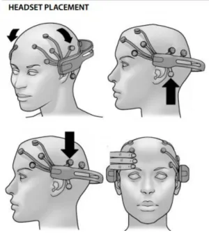
example of the EPOC/EPOC+ headset device kit with 14 electrodes that can be placed on
scalp for signal recording.
Figure 3.1. EPOC/EPOC+ headset device with 14 electrodes. Image from EMOTIV
EPOC User Manual.
The recording system can be used in different environments so the data can be collected
range [86]. The company designs the product for use in brain training and video games and
researchers have used the device in neurofeedback and raw EEG signal recording outside of
[image:46.612.155.455.272.607.2]standard laboratories [4] [14] [85].
Figure 3.2. EPOC/EPOC+ headset placement demonstration. Image from EMOTIV
3.3.2 Data Preprocessing
The collected raw EEG data is pre-processed by using EEGLAB, an interactive Matlab
toolbox for processing continuous and event-related EEG data [84]. After the pre-processing,
the EEG dataset will become a matrix with sizen×T, where n is the number of electrodes
(in our EEG recording, n= 14), and T is the total number of time points in the recording.
The dataset is saved in text file.
3.4 Experimental Results
In this section, four settings of experiments are designed and EEG data are collected in
different sessions separately. The first design has 3 minutes’ EEG and 6 blocks of activities,
each of them lasts for 30 seconds; the second design has 4 minutes’ recording and 4 blocks of
activities, each of them lasts for 1 minute; The third design has 2 minutes and 30 seconds’
EEG and 4 blocks of activities (30 seconds, 30 seconds, 1 minute and 30 seconds each); and
the last design also has 4 minutes’ recording and 4 blocks of activities, each of them lasts
for 1 minute. All experiment designs show good results after we apply the BCCPM model,
which allows us to use BCCPM in detecting change points in EEG data in additional to
fMRI data on which the BCCPM was original designed and validated.
Note that in BCCPM, there is one tuning parameter p in the program allowing us to
try different values to detect change points with different sensitivity. By default, thepis set
to be 0, if we increase p to positive values, there will be more change points detected from
the EEG data; if we decreasep to negative values, say -1000, -2000, etc., there will be fewer
change points detected. In the experimental data, choosing the optimalp is also of interest,
so multiple values has been applied: 0, -1000, -2000, -4000, -6000. We start from 0 because
there are already more than wanted change points detected at this level. Also note that we
• The second 30 seconds: solve basic mathematical operations problems in mind
• The third 30 seconds: read paragraphs from a novel
• Repeat the first 30 seconds: listen to music
• Repeat the second 30 seconds: solve basic mathematical operations problems in mind
• Repeat the third 30 seconds: read paragraphs from a novel
Table 3.1. Experiment 1 (in seconds)
0 - 30 30 - 60 60 - 90 90 - 120 120 - 150 150 - 180
music math novel music math novel
The secondsetting has 4 minutes recording with the following activities (Table 3.2):
• The first minute: listen to music
• The second minute: read paragraphs from a novel
• Repeat the first minute: listen to music
• Repeat the second minute: read paragraphs from a novel
Table 3.2. Experiment 2 (in minutes)
0 - 1 1 - 2 2 - 3 3 - 4
The third setting has 2 minutes and 30 seconds recording with the following activities
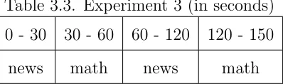
(summary shown in Table 3.3):
• The first 30 seconds: listen to live news on the radio
• The second 30 seconds: solve basic mathematical operations problems in mind
• Another one minute: listen to live news on the radio (minor change rather than
re-peating for the same time period)
• Repeat the second 30 seconds: solve basic mathematical operations problems in mind
Table 3.3. Experiment 3 (in seconds)
0 - 30 30 - 60 60 - 120 120 - 150
news math news math
The fourth setting has 4 minutes recording with the following activities (Table 3.4):
• The first minute: listen to live news on the radio
• The second minute: solve basic mathematical operations problems in mind
• Repeat the first minute: listen to live news on the radio
[image:49.612.208.407.307.366.2]• Repeat the second minute: solve basic mathematical operations problems in mind
Table 3.4. Experiment 4 (in minutes)
0 - 1 1 - 2 2 - 3 3 - 4
-2000, the number of change points decreases accordingly.
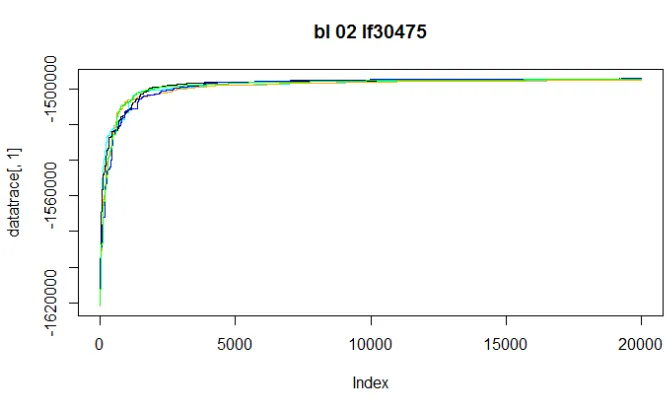
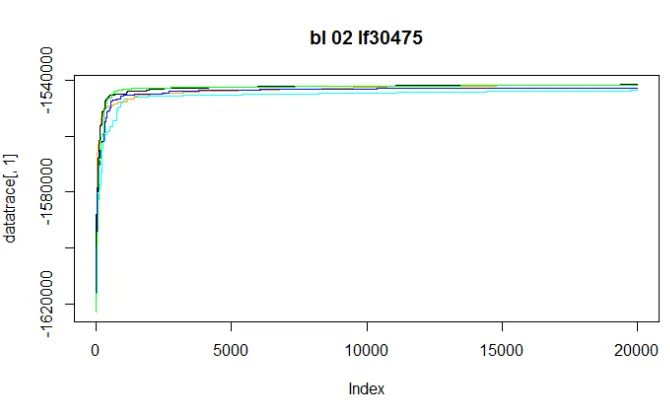
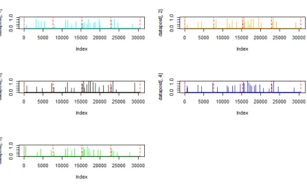
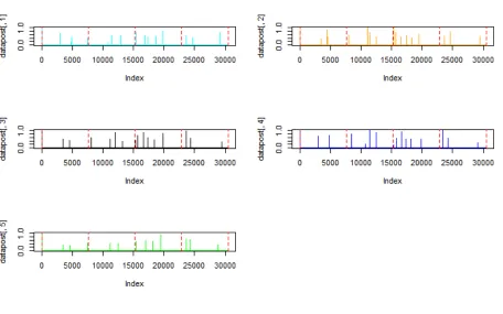
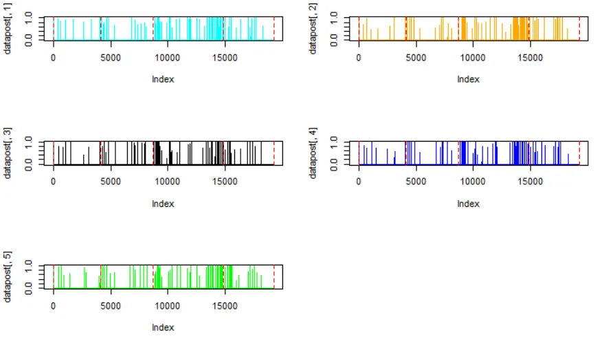
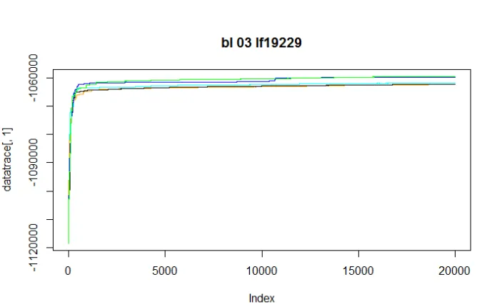
Results of the first experiment are shown in Figures 3.3 to 3.13. When p = 0, the
convergence of the markov chains are shown in Figure 3.3 and the change points detected
by BCCPM are shown in Figure 3.4. The top left plot in Figure 3.4 has the best result
according to the convergence trace plot (highest curve) and it’s enlarged as in Figure 3.5.
Now let’s take Figure 3.5 as an example, right before or after each of the red dotted lines
(locations of the designed change points), there is always a spike, which indicates a change
point detected by BCCPM at that location. At the same time, we may also observe there are
many other spikes, which are change points detected within each block atp= 0. Those could
be simply the change of brain activity related to specific task within each designed activity
block, and the number will decrease as p goes to -1000, -2000,..., -6000. When p =−1000,
the results are shown in Figures 3.6 to 3.8. Now we can observe that the number of change
points decreases. When p=−2000, the results are shown in Figures 3.9 to 3.11, the number
of change points keeps decreasing to an optimal stage where we can observe the change point
pattern much more clearly. In this study, we keep decreasing the p to -4000 and -6000, to
show that the model can detect the actual designed change points without other possible
change points not directly related to the designed blocks; for simplicity, only the best results
are shown in Figures 3.12 to 3.13. Other figures are listed in Appendix A from A.1 to A.4.
Results of the second experiment are shown in Figure 3.14 to 3.24, A.5 to A.8; results
of the third experiment are shown in Figure 3.25 to 3.35, A.9 to A.12; and results of the
Figure 3.3. Experiment 1: Traceplot shows the convergence of MCMC chains (p=0).
Figure 3.4. Experiment 1: Change points detected by BCCPM for five repeated MCMC
[image:51.612.82.525.360.642.2]Figure 3.5. Experiment 1: Change points detected by BCCPM for the best detection result
(p=0). Red dotted lines are the locations of designed change points.
Figure 3.7. Experiment 1: Change points detected by BCCPM for five repeated MCMC
chains (p=-1000). Red dotted lines are the locations of designed change points.
Figure 3.8. Experiment 1: Change points detected by BCCPM for the best detection result
Figure 3.9. Experiment 1: Traceplot shows the convergence of MCMC chains (p=-2000).
Figure 3.10. Experiment 1: Change points detected by BCCPM for five repeated MCMC
Figure 3.11. Experiment 1: Change points detected by BCCPM for the best detection
result (p=-2000). Red dotted lines are the locations of designed change points.
Figure 3.12. Experiment 1: Change points detected by BCCPM for the best detection
result (p=-4000). Red dotted lines are the locations of designed change points.
Figure 3.13. Experiment 1: Change points detected by BCCPM for the best detection
Figure 3.14. Experiment 2: Traceplot shows the convergence of MCMC chains (p=0).
Figure 3.15. Experiment 2: Change points detected by BCCPM for five repeated MCMC
[image:56.612.80.527.360.649.2]Figure 3.16. Experiment 2: Change points detected by BCCPM for the best detection
result (p=0). Red dotted lines are the locations of designed change points.
Figure 3.18. Experiment 2: Change points detected by BCCPM for five repeated MCMC
[image:58.612.78.525.79.362.2]chains (p=-1000). Red dotted lines are the locations of designed change points.
Figure 3.19. Experiment 2: Change points detected by BCCPM for the best detection
Figure 3.20. Experiment 2: Traceplot shows the convergence of MCMC chains (p=-2000).
Figure 3.21. Experiment 2: Change points detected by BCCPM for five repeated MCMC
[image:59.612.75.531.365.650.2]Figure 3.22. Experiment 2: Change points detected by BCCPM for the best detection
result (p=-2000). Red dotted lines are the locations of designed change points.
Figure 3.23. Experiment 2: Change points detected by BCCPM for the best detection
result (p=-4000). Red dotted lines are the locations of designed change points.
Figure 3.24. Experiment 2: Change points detected by BCCPM for the best detection
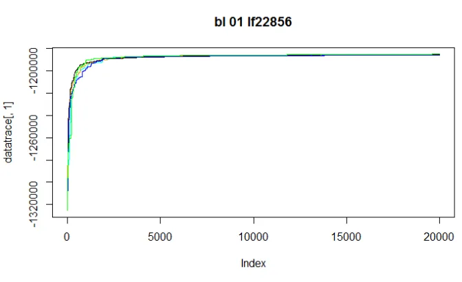
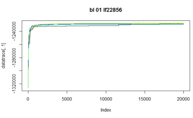
Figure 3.25. Experiment 3: Traceplot shows the convergence of MCMC chains (p=0).
Figure 3.26. Experiment 3: Change points detected by BCCPM for five repeated MCMC
Figure 3.27. Experiment 3: Change points detected by BCCPM for the best detection
result (p=0). Red dotted lines are the locations of designed change points.
Figure 3.29. Experiment 3: Change points detected by BCCPM for five repeated MCMC
[image:63.612.71.526.91.368.2]chains (p=-1000). Red dotted lines are the locations of designed change points.
Figure 3.30. Experiment 3: Change points detected by BCCPM for the best detection
Figure 3.31. Experiment 3: Traceplot shows the convergence of MCMC chains (p=-2000).
Figure 3.32. Experiment 3: Change points detected by BCCPM for five repeated MCMC
Figure 3.33. Experiment 3: Change points detected by BCCPM for the best detection
result (p=-2000). Red dotted lines are the locations of designed change points.
Figure 3.34. Experiment 3: Change points detected by BCCPM for the best detection
result (p=-4000). Red dotted lines are the locations of designed change points.
Figure 3.35. Experiment 3: Change points detected by BCCPM for the best detection
Figure 3.36. Experiment 4: Traceplot shows the convergence of MCMC chains (p=0).
Figure 3.37. Experiment 4: Change points detected by BCCPM for five repeated MCMC
Figure 3.38. Experiment 4: Change points detected by BCCPM for the best detection
result (p=0). Red dotted lines are the locations of designed change points.
Figure 3.40. Experiment 4: Change points detected by BCCPM for five repeated MCMC
[image:68.612.75.528.92.371.2]chains (p=-1000). Red dotted lines are the locations of designed change points.
Figure 3.41. Experiment 4: Change points detected by BCCPM for the best detection
Figure 3.42. Experiment 4: Traceplot shows the convergence of MCMC chains (p=-2000).
Figure 3.43. Experiment 4: Change points detected by BCCPM for five repeated MCMC
Figure 3.44. Experiment 4: Change points detected by BCCPM for the best detection
result (p=-2000). Red dotted lines are the locations of designed change points.
Figure 3.45. Experiment 4: Change points detected by BCCPM for the best detection
result (p=-4000). Red dotted lines are the locations of designed change points.
Figure 3.46. Experiment 4: Change points detected by BCCPM for the best detection
3.5 Results on EEG Data from Mindfulness Therapy for Dysfunctional Anxiety
Patients
After we validated the application of BCCPM towards EEG data through experimental
designs, we finally applied the model to our real data analysis. Results indicate that: 1)
as the mindfulness therapy goes from session 1 to later sessions, the change points in EEG
data from the subjects are decreasing, this pattern overtime indicates the subjects become
less anxious as the therapy sessions goes on; 2) At the same time, with paired data analysis,
we observe that the change-point patterns are different for different subjects in the same
session. This implies that the dynamics change is with response to treatment.
3.5.1 Recorded Data Description
In the study, there are 8 pairs of subjects in multiple mindfulness therapy sessions. A
list of paired subjects is shown in Table 3.5 with recording date, subject number and session
[image:71.612.196.415.435.695.2]number.
Table 3.5. List of paired subjects Recording Date Subject Session
10/26/2015 1001 1
1003 1
11/02/2015 1002 2
1006 2
11/30/2015 1002 5
1005 5
12/07/2015 1002 6
1006 6
12/14/2015 1001 7
1005 7
02/01/2016 1012 1
1013 1
02/22/2016 1009 4
1012 4
03/21/2016 1012 8
pattern overtime indicates the subjects become less anxious as the therapy sessions goes on.
This can be shown in Figure 3.47, as the therapy session goes on from 1 to 4 to 7 for subject
1, the number of change points decreases, which indicates that as the therapy continues,
the subject become less anxious in terms of brain activities changes. The same trend is
[image:72.612.176.434.338.655.2]discovered in all the subjects. Note that in this section, p is set at -2000 for best results.
Figure 3.47. Comparison of number of change points of Subject 1 from therapy session 1 to
In order to measure this trend quantitatively, we used Poisson process and estimated the
parameter rate which can be interpreted as the average number of points per some unit of
extents such as length, area, volumn, or time (which is our case). The Poisson rate describes
the average number of change points per time in our study and the results are summarized
in Table 3.6. We can see that the rate decreases for each subject as session goes on for all
[image:73.612.197.405.250.550.2]the subjects (except for subject 1006). The standard errors are shown in round brackets ().
Table 3.6. Poisson rates of test subjects in different sessions (p=-2000).
Subject Session Rate
(Std. Error)
1001 1 0.00075
(0.00031)
1001 4 0.00050
(0.00025)
1001 7 0.00025
(0.00018)
1002 2 0.000625
(0.00028)
1002 5 0.000375
(0.00022)
1005 5 0.00125
(0.0004)
1005 7 0.000875
(0.00033)
1006 2 0.0005
(0.00025)
1006 6 0.0005
(0.00025)
Second, the change-point patterns are different for two subjects in the same session.
This implies that the dynamics change is with response to treatment. An example is shown
in Figure 3.48. For Subject 1 and Subject 5 in session 7, the change point patterns are quite
different, which implies the change points are not associated with the therapy instructions
given by the therapist, instead it shows the true brain activities changes of the individual
Figure 3.48. In session 7, Subject 1 and Subject 5 have different change point patterns
(p=-2000).
3.6 Summary
In this chapter, we successfully extend the application of the Bayesian connectivity
change point detection model (BCCPM) onto the change point analysis of
Electroencephalog-raphy (EEG) data to determine network dynamics over time. The ability of EEG measures
of frontal and temporo-parietal activity during mindfulness therapy to track response to
treatment as preliminary evaluation for EEG as a physiological aid in therapy is successfully
CHAPTER 4
AN OPTIMIZED BAYESIAN FUNCTIONAL CONNECTIVITY CHANGE
POINT MODEL WITH GENETIC ALGORITHM
The material in this chapter is from the author’s research articles [98][97].
This research was supported by the Brains-Behavior Seed grant and Molecular Basis of
Disease(MBD) from Georgia State University. It’s a collaborative work with Dr. Xiuchun
Xiao, Dr. Jing Zhang, Dr. Yi Pan and Xueli Xiao.
The paper [98] is to appear in the Journal of Computational Biology; Xiuchun Xiao
and Bing Liu are joint first authors, and Jing Zhang and Yi Pan are joint corresponding
authors of this paper. The paper [97] has been published and can be found at https:
//doi.org/10.1007/978-3-319-59575-7_28 .
4.1 Introduction
Understanding functional localizations and exploring functional interactions within the
brain is an ongoing challenge in the area of neuroscience [68][52]. Among several methods,
neuroimaging is an efficient way to achieve this task. Functional magnetic resonance
imag-ing(fMRI) is a functional neuroimaging method [92]. By quantifying blood flow using MRI
technology, fMRI data can be used to measure human brain activities [92][22][51].
In the recent years, multiple neuroscience researches on neuronal network-level
activi-ties using fMRI dataset have invoked increasing number of attentions [101][66]. Modeling
functional connectivity and abrupt boundaries among regions of interest(ROIs) in fMRI data
has been generally considered as a powerful way to investigate brain functional interactions
[67][101][64][57].
Inspired by the successes of signal analysis technologies, sliding time window,